9.5 Viscosity

Viscocity

Most of the fluids are not ideal ones and offer some resistance to motion. This resistance to fluid motion is like an internal friction analogous to friction when a solid moves on a surface. It is called viscosity.

A real fluid flowing in a pipe experiences frictional forces. There is friction with the walls of the pipe, and there is friction within the fluid itself, converting some of its kinetic energy into thermal energy. The frictional forces that try to prevent different layers of fluid from sliding past each other are called viscous forces. Viscosity is a measure of a fluids resistance to relative motion within the fluid. We can measure the viscosity of a fluid by measuring the viscous drag between two plates.

Friction during liquid flow (fluid friction) happens due to viscosity, which is the internal resistance caused by molecules bumping, rubbing, and dragging against each other, as well as against pipe walls. This energy-dissipating interaction occurs because different layers of the fluid move at different speeds.

Lets us assume layer-1 is located at a distance \(x\) from fixed surface and its velocity is \(v\). Layer-2 is located at a distance of \(x+dx\) and its velocity is \( v+dv\). According to Newton, the frictional force \(F\) (or viscous force) between two layers depends upon the following factors:
(i) Force \(F\) is directly proportional to the area \((A)\) of the layers in contact, i.e. \(F \propto A\).
(ii) Force \(F\) is directly proportional to the velocity gradient \(\left(\frac{d v}{d x}\right)\) between the layers.
Combining these two, we have
\(
F \propto A \frac{d v}{d x}
\)
\(
F=-\eta A \frac{d v}{d x}
\)
Here, \(\eta\) is a constant of proportionality and is called coefficient of viscosity. Its value depends on the nature of the fluid.
The negative sign in the above equation shows that the direction of viscous force \(F\) is opposite to the direction of the relative velocity of the layer.
The SI unit of \(\eta\) is \(\mathrm{Nsm}^{-2}\). It is also called decapoise or pascal second.
Thus, \(\quad 1\) decapoise \(=1 \mathrm{Nsm}^{-2}=1 \mathrm{~Pa}-\mathrm{s}=10\) poise
Dimensions of \(\eta\) are \(\left[\mathrm{ML}^{-1} \mathrm{~T}^{-1}\right]\).
Coefficient of viscosity of water at \(10^{\circ} \mathrm{C}\) is \(\eta=1.3 \times 10^{-3} \mathrm{Nsm}^{-2}\). Experiments show that the coefficient of viscosity of a liquid decreases as its temperature rises.

Liquids have different viscosities depending on their properties (shown in the figure below). If you have a range of liquids at the same temperature some like water will have a low viscosity of around 1, while others like honey will have a higher viscosity of over 2000.

Example 1: A plate of area \(2 m^2\) is made to move horizontally with a speed of \(2 \mathrm{~ms}^{-1}\) by applying a horizontal tangential force over the free surface of a liquid. The depth of the liquid is 1 m and the liquid in contact with the bed is stationary. Coefficient of viscosity of liquid is 0.01 poise. Find the tangential force needed to move the plate.

Solution:

Velocity gradient \(=\frac{2-0}{1-0}=2 \mathrm{~s}^{-1}\)
From Newton’s law of viscous force,
\(
\begin{aligned}
|F| & =\eta A \frac{\Delta v}{\Delta y}=\left(0.01 \times 10^{-1}\right) \\
& =4 \times 10^{-3} \mathrm{~N}
\end{aligned}
\)
So, to keep the plate moving a force of \(4 \times 10^{-3} \mathrm{~N}\) must be applied.

Note: \(\eta=0.01 \times 0.1=0.001 \mathrm{~Pa} \cdot \mathrm{~s}=10^{-3} \mathrm{~kg} \cdot \mathrm{~m}^{-1} \cdot \mathrm{~s}^{-1}\)

Viscosity Explanation Alternate Way:

This force exists when there is relative motion between layers of the liquid. Suppose we consider a fluid like oil enclosed between two glass plates as shown in Figure below. The bottom plate is fixed while the top plate is moved with a constant velocity \({v}\) relative to the fixed plate. If oil is replaced by honey, a greater force is required to move the plate with the same velocity. Hence we say that honey is more viscous than oil. The fluid in contact with a surface has the same velocity as that of the surfaces. Hence, the layer of the liquid in contact with top surface moves with a velocity \({v}\) and the layer of the liquid in contact with the fixed surface is stationary. The velocities of layers increase uniformly from bottom (zero velocity) to the top layer (velocity \(v\)). For any layer of liquid, its upper layer pulls it forward while lower layer pulls it backward. This results in force between the layers. This type of flow is known as laminar. The layers of liquid slide over one another as the pages of a book do when it is placed flat on a table and a horizontal force is applied to the top cover. When a fluid is flowing in a pipe or a tube, then velocity of the liquid layer along the axis of the tube is maximum and decreases gradually as we move towards the walls where it becomes zero.

On account of this motion (as shown with arrow in diagram below), a portion of liquid, which at some instant has the shape \(A B C D\), take the shape of AEFD after short interval of time ( \(\Delta t\) ). During this time interval the liquid has undergone a shear strain of \(\Delta x / l\). Since, the strain in a flowing fluid increases with time continuously. Unlike a solid, here the stress is found experimentally to depend on ‘rate of change of strain’ or ‘strain rate’ i.e. \(\Delta x /(l \Delta t)\) or \(v / l\) instead of strain itself.

The coefficient of viscosity (pronounced ‘eta’) for a fluid is defined as the ratio of shearing stress to the strain rate.
\(
\eta=\frac{\text { shearing stress }}{ \text { strain rate }}=\frac{F / A}{v / l}=\frac{F l}{v A}
\)

Note: Strain rate is a measure of how quickly a material deforms or changes shape over time. Shear strain is the deformation of an object that occurs when a force acts parallel to its surface.
Strain rate = (Change in strain) / (Change in time)=\(\Delta x / l / (\Delta t)=\Delta x /(l \Delta t)=v/l\)
Strain rate is represented by the formula “\(v/l\)“, where ” \(v\) ” is the velocity and “\(l\)” is the length, meaning it calculates the rate of deformation by dividing the change in length by the original length per unit time; essentially, how fast a material is changing shape relative to its original size.

Example 2: A metal block of area \(0.10 \mathrm{~m}^2\) is connected to a 0.010 kg mass via a string that passes over an ideal pulley (considered massless and frictionless) as shown below. A liquid with a film thickness of 0.30 mm is placed between the block and the table. When released the block moves to the right with a constant speed of \(0.085 \mathrm{~m} \mathrm{~s}^{-1}\). Find the coefficient of viscosity of the liquid.

Solution: The metal block moves to the right because of the tension in the string. The tension \(T\) is equal in magnitude to the weight of the suspended mass \(m\). Thus, the shear force \(F\) is
\(
F=T=m g=0.010 \mathrm{~kg} \times 9.8 \mathrm{~m} \mathrm{~s}^{-2}=9.8 \times 10^{-2} \mathrm{~N}
\)
Shear stress on the fluid \(=F / A=\frac{9.8 \times 10^{-2}}{0.10} \mathrm{~N} / \mathrm{m}^2\)
\(
\begin{aligned}
& \text { Strain rate }=\frac{v}{l}=\frac{0.085}{0.30 \times 10^{-3}} \\
& \eta=\frac{\text { stress }}{\text { strain rate }} \mathrm{s}^{-1} \\
& =\frac{\left(9.8 \times 10^{-2} \mathrm{~N}\right)\left(0.30 \times 10^{-3} \mathrm{~m}\right)}{\left(0.085 \mathrm{~m} \mathrm{~s}^{-1}\right)\left(0.10 \mathrm{~m}^2\right)} \\
& =3.46 \times 10^{-3} \mathrm{~Pa} \mathrm{~s}
\end{aligned}
\)

Stokes’ Law

When an object moves through a fluid, it experiences a viscous force which acts in opposite direction of its velocity. It is seen that the viscous force is proportional to the velocity of the object and is opposite to the direction of motion. The other quantities on which the force \(F\) depends are viscosity \(\eta\) of the fluid and radius \(r\) of the sphere. Sir George G. Stokes (1819-1903), an English scientist enunciated clearly the viscous drag force \(F\) as
\(F=6 \pi \eta r v\) (where, \(\eta=\) coefficient of viscosity)
This law is called Stokes’ law.

Proof: Step 1: The Definition of Viscous Force
Recall that for a fluid layer, the viscous force \(F\) is defined as:
\(
F=\eta A \frac{d v}{d y}
\)
\(\eta\) : Coefficient of viscosity.
A: The area of the surface in contact with the fluid.
\(\frac{d v}{d y}\) : The velocity gradient (how fast the fluid speed changes as you move away from the object).
STep 2: Applying this to a Sphere
When a sphere of radius \(r\) moves through a fluid at velocity \(v\), we need to estimate the “effective” area and the “effective” velocity gradient.
The Area \((A)\) : The surface area of a sphere is \(4 \pi r^2\). So, \(A\) is proportional to \(r^2\).
The Velocity Gradient \(\left(\frac{d v}{d y}\right)\) : * Right at the surface of the sphere, the fluid moves at velocity \(v\).
Far away, the fluid is still (velocity \(=0\)).
The distance over which this change happens is roughly the radius of the sphere, \(r\).
Therefore, the gradient is approximately \(\frac{v}{r}\).
Step 3: Combining the Terms
Now, let’s plug these approximations into the general force equation:
\(
\begin{gathered}
F \approx \eta \cdot(\text { Area }) \cdot(\text { Velocity Gradient }) \\
F \approx \eta \cdot\left(r^2\right) \cdot\left(\frac{v}{r}\right)
\end{gathered}
\)
Simplifying this gives:
\(
F \approx \eta r v
\)
Step 4: The Geometry Constant
The “rough” derivation above gives us the variables, but it doesn’t give us the exact number. To get the \(6 \pi\), you have to account for:
Pressure Drag: The difference in pressure between the front and back of the sphere ( \(2 \pi \eta r v)\).
Friction Drag: The actual rubbing of the fluid against the sides (\(4 \pi \eta r v\)).
Adding these two distinct physical effects together gives the complete Stokes’ Law:
\(
F=6 \pi \eta r v
\)

Terminal velocity \(\left(v_t\right)\)

This law is an interesting example of retarding force, which is proportional to velocity. We can study its consequences on an object falling through a viscous medium. We consider a raindrop in air. It accelerates initially due to gravity. As the velocity increases, the retarding force also increases. Finally, when viscous force plus buoyant force becomes equal to the force due to gravity, the net force becomes zero and so does the acceleration. The sphere (raindrop) then descends with a constant velocity. Thus, in equilibrium, this velocity is known as terminal velocity \(v_{\mathrm{t}}\).

Consider a small sphere falling from rest through a large column of viscous fluid.

The forces acting on the sphere are
(i) weight \(w\) of the sphere acting vertically downwards.
(ii) upthrust buoyant force \(F_t\) acting vertically upwards.
(iii) viscous force \(F_v\) acting vertically upwards, i.e. in a direction opposite to velocity of the sphere.
Initially,
\(
\begin{aligned}
F_v & =0  \quad (\because v=0) \\
w & >F_t
\end{aligned}
\)
and the sphere accelerates downwards. As the velocity of the sphere increases, \(F_v\) increases. Eventually, a stage is reached when
\(
w=F_t+F_v \dots(i)
\)
After this net force on the sphere is zero and it moves downwards with a constant velocity called terminal velocity \(\left(v_t\right)\).
It can be defined as the maximum constant velocity acquired by a body while falling through a viscous medium.

Substituting proper values in Eq. (i), we get
\(
\frac{4}{3} \pi r^3 \rho g=\frac{4}{3} \pi r^3 \sigma g+6 \pi \eta r v_t \dots(ii)
\)
Here, \(\quad \rho=\) density of sphere, \(\sigma=\) density of fluid and \(\quad \eta=\) coefficient of viscosity of fluid.
From Eq. (ii), we get
\(
v_t=\frac{2}{9} \frac{r^2(\rho-\sigma) g}{\eta}
\)
The figure shows the variation of the velocity \(v\) of the sphere with time

Note: From the above expression, we can see that the terminal velocity of a spherical body is directly proportional to the difference in the densities of the body and the fluid \((\rho-\sigma)\). If the density of the fluid is greater than that of body (i.e. \(\sigma>\rho\) ), the terminal velocity is negative. This means that the body instead of falling, moves upward. This is why air bubbles rise up in water.

Example 3: The terminal velocity of a copper ball of radius 2.0 mm falling through a tank of oil at \(20^{\circ} \mathrm{C}\) is \(6.5 \mathrm{~cm} \mathrm{~s}^{-1}\). Compute the viscosity of the oil at \(20^{\circ} \mathrm{C}\). Density of oil is \(1.5 \times 10^3 \mathrm{~kg} \mathrm{~m}^{-3}\), density of copper is \(8.9 \times 10^3 \mathrm{~kg} \mathrm{~m}^{-3}\).

Solution: We have \(v_{\mathrm{t}}=6.5 \times 10^{-2} \mathrm{~ms}^{-1}, r=2 \times 10^{-3} \mathrm{~m}\), \(g=9.8 \mathrm{~ms}^{-2}, \rho=8.9 \times 10^3 \mathrm{~kg} \mathrm{~m}^{-3}\), \(\sigma=1.5 \times 10^3 \mathrm{~kg} \mathrm{~m}^{-3}\). We know
\(
v_{\mathrm{t}}=2 r^2(\rho-\sigma) g /(9 \eta)
\)
\(
\begin{aligned}
\eta & =\frac{2}{9} \times \frac{\left(2 \times 10^{-3}\right)^2 \mathrm{~m}^2 \times 9.8 \mathrm{~m} \mathrm{~s}^{-2}}{6.5 \times 10^{-2} \mathrm{~m} \mathrm{~s}^{-1}} \times 7.4 \times 10^3 \mathrm{~kg} \mathrm{~m}^{-3} \\
& =9.9 \times 10^{-1} \mathrm{~kg} \mathrm{~m}^{-1} \mathrm{~s}^{-1}
\end{aligned}
\)

Example 4: With what terminal velocity will an air bubble 0.8 mm in diameter rise in a liquid of viscosity \(0.15 \mathrm{Nsm}^{-2}\) and specific gravity \(0.9 \mathrm{kgm}^{-3}\)? (Take, the density of air is \(1.293 \mathrm{~kg} \mathrm{~m}^{-3}\) )

Solution: The terminal velocity of the bubble is given by
\(
v_t=\frac{2}{9} \frac{r^2(\rho-\sigma) g}{\eta}
\)
Here,
\(
\begin{aligned}
& r=0.4 \times 10^{-3} \mathrm{~m}, \sigma=0.9 \times 10^3 \mathrm{kgm}^{-3} \\
& \rho=1.293 \mathrm{kgm}^{-3}, \eta=0.15 \mathrm{Nsm}^{-2}
\end{aligned}
\)
and \(\quad g=9.8 \mathrm{~ms}^{-2}\)
Substituting the values, we get
\(
\begin{aligned}
v_t & =\frac{2}{9} \times \frac{\left(0.4 \times 10^{-3}\right)^2\left(1.293-0.9 \times 10^3\right) \times 9.8}{0.15} \\
& =-0.0021 \mathrm{~ms}^{-1} \text { or } v_t=-0.21 \mathrm{cms}^{-1}
\end{aligned}
\)
Note Here, a negative sign implies that the bubble will rise up.

Example 5: Two spherical raindrops of equal size are falling vertically through air with a terminal velocity of \(1 \mathrm{~ms}^{-1}\). What would be the terminal speed, if these two drops were to coalesce to form a large spherical drop?

Solution: As,
\(
v_t \propto r^2
\)
Let \(r\) be the radius of small raindrops and \(R\) the radius of large drop.
Equating the volumes, we get
\(
\begin{aligned}
& & \frac{4}{3} \pi R^3 & =2\left(\frac{4}{3} \pi r^3\right) \\
& \therefore & R & =(2)^{1 / 3} \cdot r \text { or } \frac{R}{r}=(2)^{1 / 3} \\
& \because & \frac{v_t^{\prime}}{v_t} & =\left(\frac{R}{r}\right)^2=(2)^{2 / 3} \\
& \therefore & v_t^{\prime} & =(2)^{2 / 3}(1.0) \mathrm{ms}^{-1}=1.587 \mathrm{~ms}^{-1}
\end{aligned}
\)

Flow of liquid through a cylindrical pipe

Figure shows the flow speed profile for laminar flow of a viscous fluid in a long cylindrical pipe. The speed is greatest along the axis and zero at the pipe walls.

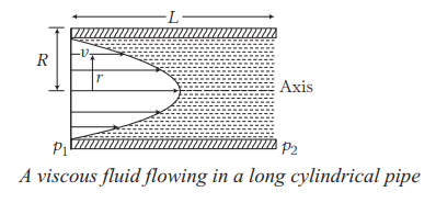
To derive the velocity profile for laminar flow in a pipe-commonly known as Poiseuille Flow, we look at the balance of forces acting on a cylindrical element of fluid.
Define the System:
Imagine a horizontal pipe of radius \(R\) and length \(L\). We consider a small cylindrical “plug” of fluid inside the pipe with radius \(r\) and length \(L\), concentric with the pipe’s axis.
Two main forces act on this fluid element:
Pressure Force: Pushing the fluid forward.
Viscous (Friction) Force: Resisting the motion at the surface of the cylinder.
Since the flow is steady (no acceleration), the net force must be zero.
Pressure Force \(\left(F_p\right)\) : The pressure \(p_1\) acts on the left face and \(p_2\) on the right. The crosssectional area is \(\pi r^2\).
\(
F_p=\left(p_1-p_2\right) \pi r^2
\)
Viscous Force \(\left(F_v\right)\) : According to Newton’s law of viscosity, the shear stress \(\tau\) is \(\eta \frac{d v}{d r}\). This stress acts on the surface area of the cylinder \((2 \pi r L)\).
\(
F_v=\tau \cdot(2 \pi r L)=\eta \frac{d v}{d r}(2 \pi r L)
\)
Setting the forces equal (in magnitude):
\(
\left(p_1-p_2\right) \pi r^2=-\eta \frac{d v}{d r}(2 \pi r L)
\)
(Note: We use a negative sign because the velocity \(v\) decreases as the radius \(r\) increases.)
Now, we rearrange the equation to solve for \(d v\) :
\(
d v=-\frac{p_1-p_2}{2 \eta L} r d r
\)
To find the velocity \(v\) at a distance \(r\), we integrate from the pipe wall (where the fluid is stationary) to the distance \(r\).
Boundary Condition: At \(r=R, v=0\) (the “no-slip” condition).
\(
\int_0^v d v=-\frac{p_1-p_2}{2 \eta L} \int_R^r r d r
\)
Evaluating the integral:
\(
\begin{gathered}
v=-\frac{p_1-p_2}{2 \eta L}\left[\frac{r^2}{2}\right]_R^r \\
v=-\frac{p_1-p_2}{4 \eta L}\left(r^2-R^2\right)
\end{gathered}
\)
Final Equation:
By distributing the negative sign, we reach the standard form:
\(
v=\frac{p_1-p_2}{4 \eta L}\left(R^2-r^2\right)
\)
This shows that the velocity profile is parabolic, with the maximum velocity occurring at the center \((r=0)\) and zero velocity at the walls \((r=R)\).

Volume flow rate \(\left(Q\right.\) or \(\left.\frac{d V}{d t}\right)\) : Poiseuille equation

The result is \(Q=\frac{d V}{d t}=\frac{\pi}{8}\left(\frac{R^4}{\eta}\right)\left(\frac{p_1-p_2}{L}\right)\)

Derivation:

To explain this derivation clearly, it helps to visualize the fluid not as a single mass, but as a series of concentric “cylindrical shells” sliding past one another.
Why use a “Ring” (\(dA\))?
we pick a tiny, representative “ring” at radius \(r\).
The velocity \(v(r)\) is constant everywhere on this specific ring.
The area of this ring is its circumference \((2 \pi r)\) multiplied by its infinitesimal thickness \((d r\)), giving us \(d A=2 \pi r d r\).
The Setup of the Integral:
The volume flow rate (\(d Q\)) through that single tiny ring is:
\(
d Q=v(r) \cdot d A
\)
Substituting the velocity profile \(v=\frac{p_1-p_2}{4 \eta L}\left(R^2-r^2\right)\) and the area \(d A=2 \pi r d r\) :
\(
d Q=\left[\frac{p_1-p_2}{4 \eta L}\left(R^2-r^2\right)\right] \cdot[2 \pi r d r]
\)
The Physical Integration:
To get the total flow (\(Q\)), we sum up all these rings from the center (\(r=0\)) to the outer wall (\(r=R\)).
\(
Q=\int_0^R \frac{2 \pi\left(p_1-p_2\right)}{4 \eta L}\left(R^2 r-r^3\right) d r
\)
When you perform the integration, the \(R^2 r\) term becomes \(\frac{R^2 r^2}{2}\) and the \(r^3\) term becomes \(\frac{r^4}{4}\). Plugging in the limits from 0 to \(R\) :
\(
Q=\frac{\pi\left(p_1-p_2\right)}{2 \eta L}\left(\frac{R^4}{2}-\frac{R^4}{4}\right)=\frac{\pi\left(p_1-p_2\right)}{2 \eta L}\left(\frac{R^4}{4}\right)
\)
The Poiseuille Equation: (The relation was first derived by Poiseuille and is called Poiseuille’s equation.)
\(
Q=\frac{d V}{d t}=\frac{\pi R^4\left(p_1-p_2\right)}{8 \eta L}
\)

What this tells us physically:

• \(R^4\) Dependence: This is the most critical takeaway. If you double the radius of a pipe, you don’t just get double or quadruple the flow; you get 16 times more flow \(\left(2^4=16\right)\). This explains why even a small amount of plaque in an artery significantly restricts blood flow.
• Pressure Gradient: Flow is directly proportional to the pressure drop (\(\Delta p\)) per unit length (\(L\)).
• Viscosity: Flow is inversely proportional to viscosity \((\eta)\). Thicker fluids (like motor oil) flow slower than thinner fluids (like water) under the same pressure.

Some important points related to Poiseuille equation are given below:

• Poiseuille’s equation can also be written as
  \(
  Q=\frac{p_1-p_2}{\left(\frac{8 \eta L}{\pi R^4}\right)}=\frac{\Delta p}{X} \text {, here } X=\frac{8 \eta L}{\pi R^4}
  \)
  This equation can be compared with the current equation through a resistance, i.e. \(i=\frac{\Delta V}{R}\).
  Here, \(\Delta V=\) potential difference
  and \(R=\) electrical resistance.
  For current flow through a resistance, potential difference is a requirement, similarly for flow of liquid through a pipe, pressure difference is must.
• Problems of series and parallel combination of pipes can be solved in the similar manner as is done in case of an electrical circuit. The only difference is
  (a) Potential difference \((\Delta V)\) is replaced by the pressure difference \((\Delta p)\).
  (b) The electrical resistance \(R\left(=\rho \frac{L}{A}\right)\) is replaced by flow resistance \(X\left(=\frac{8 \eta L}{\pi R^4}\right)\).
  (c) The electrical current \(i\) is replaced by volume flow rate \(Q\) or \(d V / d t\).

Combination of capillary (thin) tubes

Case-I: Series combination of Pipes

(a) The rate of flow \((Q)\) will be same.
(b) Pressure difference across each tube is different.

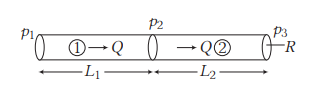
In a series circuit, the “current” (volume flow rate \(Q\)) must be the same through every section of the pipe to satisfy the conservation of mass (continuity).
The Physical Setup:
Imagine two pipes of lengths \(L_1\) and \(L_2\) joined end-to-end. The pressure at the start is \(p_1\), the junction is \(p_2\), and the exit is \(p_3\).
Deriving the Equivalent Resistance:
Just like resistors in an electrical circuit, the total pressure drop is the sum of the individual pressure drops across each section:
Pressure drop in Pipe 1: \(\Delta p_1=p_1-p_2=Q X_1\)
Pressure drop in Pipe 2: \(\Delta p_2=p_2-p_3=Q X_2\)
The Total Pressure Drop ( \(\Delta p_{\text {total }}\) ) is:
\(
\Delta p_{\text {total }}=\left(p_1-p_2\right)+\left(p_2-p_3\right)=p_1-p_3
\)
Substituting the flow equations:
\(
\Delta p_{t o t a l}=Q X_1+Q X_2=Q\left(X_1+X_2\right)
\)
Since \(\Delta p_{\text {total }}=Q X_{\text {eq }}\), we can see that:
\(
X_{e q}=X_1+X_2
\)
Case Study: Same Radius, Different Lengths:
If both pipes have the same radius \(R\) and viscosity \(\eta\), the formula simplifies beautifully as you noted:
\(
X_{e q}=\frac{8 \eta L_1}{\pi R^4}+\frac{8 \eta L_2}{\pi R^4}=\frac{8 \eta}{\pi R^4}\left(L_1+L_2\right)
\)
This proves that two pipes of length \(L_1\) and \(L_2\) in series behave exactly like a single pipe of length \(\left(L_1+L_2\right)\).

Summary: Series Pipes
\(
\begin{array}{llll}
\text { Feature } & \text { Pipe } 1 & \text { Pipe } 2 & \text { Combined (Series) } \\
\text { Flow Rate } & Q & Q & Q \text { (Same everywhere) } \\
\text { Pressure Drop } & \Delta p_1 & \Delta p_2 & \Delta p_1+\Delta p_2 \\
\text { Resistance } & X_1 & X_2 & X_1+X_2
\end{array}
\)

Case-II: Parallel combination of pipes

(a) The pressure difference across each tube is same.
(b) The rate of flow across each tube is different.

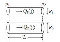
When pipes are connected in parallel, they behave exactly like resistors in an electrical circuit where the voltage (pressure) is the same across all branches, but the current (flow rate) splits.
The Physical Principles:
Imagine a single pipe splitting into two separate branches (Tube 1 and Tube 2 ) and then recombining.
Pressure (\(\Delta p\)): Since both tubes start at the same point (\(p_1\)) and end at the same point (\(\left.p_2\right)\), the pressure difference \(\Delta p=p_1-p_2\) is identical for every tube in the parallel network.
Flow Rate (Q): The total fluid entering the junction must equal the sum of the fluid traveling through each branch.
\(
Q_{\text {total }}=Q_1+Q_2
\)
Deriving Equivalent Resistance (\(\boldsymbol{X}_{\text {eq }}\)):
Using the fluid version of Ohm’s Law (\(Q=\frac{\Delta p}{X}\)), we can substitute the flow rates for each branch:
\(
Q_{\text {total }}=\frac{\Delta p}{X_1}+\frac{\Delta p}{X_2}
\)
Since the equivalent resistance \(X_{e q}\) must satisfy the relationship \(Q_{\text {total }}=\frac{\Delta p}{\bar{X}_{e q}}\), we can write:
\(
\frac{\Delta p}{X_{e q}}=\frac{\Delta p}{X_1}+\frac{\Delta p}{X_2}
\)
Dividing both sides by \(\boldsymbol{\Delta} \boldsymbol{p}\) gives the Parallel Resistance Formula:
\(
\frac{1}{X_{e q}}=\frac{1}{X_1}+\frac{1}{X_2}
\)
Substituting the Poiseuille Constants:
If we have two pipes of lengths \(L_1, L_2\) and radii \(R_1, R_2\), the individual resistances are \(X= \frac{8 \eta L}{\pi R^4}\). The total flow rate becomes:
\(
Q_{\text {total }}=\frac{\pi \Delta p}{8 \eta}\left(\frac{R_1^4}{L_1}+\frac{R_2^4}{L_2}\right)
\)

Summary: Series Vs Parallel Pipes:
\(
\begin{array}{lll}
\text { Feature } & \text { Series Combination } & \text { Parallel Combination } \\
\text { Flow Rate }(Q) & \text { Same for all pipes }\left(Q_1=Q_2\right) & \text { Sum of all pipes }\left(Q_{t o t}=Q_1+Q_2\right) \\
\text { Pressure Drop }(\Delta p) & \text { Sum of all pipes }\left(\Delta p_1+\Delta p_2\right) & \text { Same for all pipes }\left(\Delta p_1=\Delta p_2\right) \\
\text { Equivalent Resistance } & X_{e q}=X_1+X_2 & \frac{1}{X_{e q}}=\frac{1}{X_1}+\frac{1}{X_2}
\end{array}
\)

Example 6: Water is flowing through a horizontal tube 8 cm in diameter and 4 km in length at the rate of 20 litre/s. Assuming only viscous resistance. Find the pressure required to maintain the flow in terms of mercury column. (Take, coefficient of viscosity of water is 0.001 Pa-s)

Solution: Here, \(2 r=8 \mathrm{~cm}=0.08 \mathrm{~m}\) or \(r=0.04 \mathrm{~m}, l=4 \mathrm{~km}=4000 \mathrm{~m}\),
\(
V=20 \text { litre } / \mathrm{s}=20 \times 10^{-3} \mathrm{~m}^3 \mathrm{~s}^{-1}, \eta=0.001 \mathrm{~Pa}-\mathrm{s}, p=?
\)
As, \(\quad V=\frac{\pi p r^4}{8 \eta l}\) or \(p=\frac{8 V \eta l}{\pi r^4}\)
\(
=\frac{8 \times\left(20 \times 10^{-3}\right) \times 0.001 \times 4000}{\left(\frac{22}{7}\right) \times(0.04)^4}=7.954 \times 10^4 \mathrm{~Pa}
\)
∴ Height of mercury column for pressure difference \(p\) will be
\(
h=\frac{p}{\rho g}=\frac{7.954 \times 10^4}{\left(13.6 \times 10^3\right) \times 9.8}=0.5968 \mathrm{~m}=59.68 \mathrm{~cm}
\)

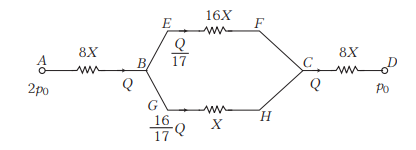
Example 7: A liquid is flowing through horizontal pipes as shown in figure.

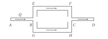
Length of different pipes has the following ratio
\(
L_{A B}=L_{C D}=\frac{L_{E F}}{2}=\frac{L_{G H}}{2}
\)
Similarly, radii of different pipes has the ratio,
\(
R_{A B}=R_{E F}=R_{C D}=\frac{R_{G H}}{2}
\)
Pressure at \(A\) is \(2 p_0\) and pressure at \(D\) is \(p_0\). The volume flow rate through the pipe \(A B\) is \(Q\). Find
(i) volume flow rates through \(E F\) and \(G H\)
(ii) pressure at \(E\) and \(F\).

Solution: The equivalent electrical circuit can be drawn as under,
\(
X \propto \frac{L}{R^4} \quad\left(\because X=\frac{8 \eta L}{\pi R^4}\right)
\)

\(
\begin{aligned}
\therefore \quad X_{A B}: X_{C D}: X_{E F}: X_{G H} & =\frac{\frac{1}{2}}{\left(\frac{1}{2}\right)^4}: \frac{\left(\frac{1}{2}\right)}{\left(\frac{1}{2}\right)^4}: \frac{(1)}{\left(\frac{1}{2}\right)^4}: \frac{(1)}{(1)^4} \\
& =8: 8: 16: 1
\end{aligned}
\)
(i) As the current is distributed in the inverse ratio of the resistance (in parallel), the \(Q\) will be distributed in the inverse ratio of \(X\).
Thus, volume flow rate through \(E F\) will be \(\frac{Q}{17}\) and that from \(G H\) will be \(\frac{16}{17} Q\).
(ii)
\(
\begin{aligned}
X_{\mathrm{net}} & =8 X+\left[\frac{(16 X)(X)}{(16 X)+(X)}\right]+8 X=\frac{288}{17} X \\
\therefore \quad Q & =\frac{\Delta p}{X_{\mathrm{net}}} \quad\left(\because i=\frac{\Delta V}{R}\right) \\
& =\frac{\left(2 p_0-p_0\right)}{\frac{288}{17} X}=\frac{17 p_0}{288 X}
\end{aligned}
\)
Now, let \(p_1\) be the pressure at \(E\), then
\(
\begin{aligned}
2 p_0-p_1 & =8 Q X=\frac{8 \times 17 p_0}{288} \\
\therefore \quad p_1 & =\left(2-\frac{17 \times 8}{288}\right) p_0 \\
& =1.53 p_0
\end{aligned}
\)
Similarly, if \(p_2\) be the pressure at \(F\), then
\(
\begin{aligned}
p_2-p_0 & =8 Q X \\
\therefore \quad p_2 & =p_0+\frac{8 \times 17}{288} p_0 \\
p_2 & =1.47 p_0
\end{aligned}
\)