8.3 Hooke’s law

For small deformations the stress and strain are proportional to each other. This is known as Hooke’s law.
Thus, stress \(\propto\) strain
stress \(=E \times\) strain
where \(E=\frac{\text { stress }}{\text { strain }}\) is the proportionality constant and is known as modulus of elasticity.
The SI unit of modulus of elasticity is \(\mathrm{Nm}^{-2}\) and its dimensions are \(\left[\mathrm{ML}^{-1} \mathrm{~T}^{-2}\right]\).
The modulus of elasticity depends on the type of material and temperature. It does not depend upon the values of stress and strain.
Depending upon the nature of force applied on the body, the modulus of elasticity is classified in the following three types:

Note: Hooke’s law is an empirical law and is found to be valid for most materials. However, there are some materials which do not exhibit this linear relationship.

Young’s modulus of elasticity \((Y)\)

The ratio of tensile stress (longitudinal) over tensile (longitudinal) strain is called Young modulus \((Y)\) for the material.
\(Y=\frac{\text { Tensile stress }}{\text { Tensile strain }}=\frac{\text { longitudinal stress }}{\text { longitudinal strain }}=\frac{\sigma}{\varepsilon}\)

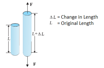
For a small change in the length of the wire, the ratio of the longitudinal stress to the longitudinal strain is called the Young’s modulus of elasticity \((Y)\) of the wire.
Thus, \(Y=\frac{\frac{F}{A}}{\frac{\Delta L}{L}}\) or \(Y=\frac{F L}{A \Delta L}\)
Let there be a wire of length \(L\) and radius \(r\). Its one end is clamped to a rigid support and a mass \(M\) is attached at the other end. Then,
\(
F=M g \text { and } A=\pi r^2
\)
Substituting in above equation, we have
\(
Y=\frac{M g L}{\left(\pi r^2\right) \Delta L}
\)
Young’s modulus is only defined for solids, and not for liquids and gases. Larger the value of \(Y\) for a material, more elastic it would be. For this reason, steel is more elastic than rubber.
The material which has smaller value of \(Y\) is more ductile, i.e. it offers less resistance in framing it into wire. Thus, for making wire, we choose a material having less value of \(Y\).
Note: For a perfectly rigid body, value of \(Y\) is infinite. A perfectly rigid body does not undergo any change in length ( \(\Delta L=0\) ) or shape when subjected to external force or stress.

Example 1: A load of 4.0 kg is suspended from a ceiling through a steel wire of length 20 m and radius 2.0 mm. It is found that the length of the wire increases by 0.031 mm as equilibrium is achieved. Find Young modulus of steel. Take \(g=3 \cdot 1 \pi \mathrm{~m} \mathrm{~s}^{-2}\).

Solution:
\(
\begin{aligned}
\text { The longitudinal stress } & =\frac{(4.0 \mathrm{~kg})\left(3.1 \pi \mathrm{~m} \mathrm{~s}^{-2}\right)}{\pi\left(2.0 \times 10^{-3} \mathrm{~m}\right)^2} \\
& =3.1 \times 10^6 \mathrm{~N} \mathrm{~m}^{-2}
\end{aligned}
\)
The longitudinal strain \(=\frac{0.031 \times 10^{-3} \mathrm{~m}}{2.0 \mathrm{~m}}\)
\(
=0.0155 \times 10^{-3}
\)
Thus \(Y=\frac{3.1 \times 10^6 \mathrm{~N} \mathrm{~m}^{-2}}{0.0155 \times 10^{-3}}=2.0 \times 10^{11} \mathrm{~N} \mathrm{~m}^{-2}\).

Force constant of wire

Force required to produce unit elongation in a wire is called force constant of material of wire. It is denoted by \(k\).
\(
k=\frac{F}{\Delta l}=\frac{Y A}{l} \quad\left(\because \frac{F}{\Delta l}=\frac{Y A}{l}\right)
\)
If a spring is stretched or compressed by an amount \(\Delta l\), the restoring force produced in it, is
\(
F_{\mathrm{s}}=k \Delta l \dots(i)
\)
Here, \(k=\) force constant of spring.
Similarly, if a wire is stretched by an amount \(\Delta l\), the restoring force produced in it, is
\(
F=\left(\frac{Y A}{l}\right) \Delta l \dots(ii)
\)
Comparing Eqs. (i) and (ii), we can see that force constant of a wire,
\(
k=\frac{Y A}{l} \dots(iii)
\)
i.e. A wire is just like a spring of force constant \(\frac{Y A}{l}\).
So, all formulae which we use in case of a spring can be applied to a wire also.

Example 2: A cable is replaced by another one of same length and material but twice the diameter. How will this effect the elongation under a given load? How does this effect the maximum load, it can support without exceeding the elastic limit?

Solution: Young’s modulus, \(Y=\frac{M g l}{\pi r^2 \cdot \Delta l}=\frac{M g l}{\pi\left(\frac{D}{2}\right)^2 \Delta l}=\frac{4 M g l}{\pi D^2 \cdot \Delta l}\) where, \(D\) is the diameter of the wire.
∴ Elongation, \(\Delta l=\frac{4 M g l}{\pi D^2 \cdot Y}\), i.e. \(\Delta l \propto \frac{1}{D^2}\)
Clearly, if the diameter is doubled, the elongation will become one-fourth.
Also, maximum stress, \(S_m=\frac{M_m g}{\left(\pi D^2 / 4\right)}\)
\(
M_m \propto D^2
\)
Clearly, if the diameter is doubled, the wire can support four times the original load.

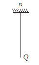
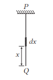
Example 3: \(A\) bar of mass \(m\) and length \(l\) is hanging from point \(A\) as shown in figure. Find the increase in its length due to its own weight. The Young’s modulus of elasticity of the wire is \(Y\) and area of cross-section of the wire is \(A\).

Solution: Consider a small section \(d x\) of the bar at a distance \(x\) from \(Q\). The weight of the bar for a length \(x\) is,
\(
w=\left(\frac{m g}{l}\right) x
\)

Elongation in section \(d x\) will be, \(d l=\left(\frac{w}{A Y}\right) d x=\left(\frac{m g}{l A Y}\right) x d x\)
Total elongation in the bar can be obtained by integrating this expression for \(x=0\) to \(x=l\).
\(
\therefore \quad \Delta l=\int_{x=0}^{x=l} d l=\left(\frac{m g}{l A Y}\right) \int_0^l x d x
\)
or Increase in length, \(\Delta l=\frac{m g l}{2 A Y}\)

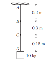
Example 4: A rod \(A D\) consisting of three segments \(A B\), \(B C\) and \(C D\) joined together is hanging vertically from a fixed support at \(A\). The lengths of the segments are respectively \(0.2 m, 0.3 m\) and \(0.15 m\). The cross-section of the rod is uniformly \(10^{-4} \mathrm{~m}^2\). A weight of 10 kg is hung from \(D\). Calculate the displacements of points \(B\), \(C\) and \(D\), if \(Y_{A B}=3.5 \times 10^{10} \mathrm{Nm}^{-2}, Y_{B C}=5 \times 10^{10} \mathrm{Nm}^{-2}\), \(Y_{C D}=2 \times 10^{10} \mathrm{Nm}^{-2}\). (Neglect the weight of the rod).

Solution: Given, area, \(A=10^{-4} \mathrm{~m}^2\),
\(
\begin{aligned}
Y_{A B} & =3.5 \times 10^{10} \mathrm{Nm}^{-2} \\
Y_{B C} & =5 \times 10^{10} \mathrm{Nm}^{-2} \\
Y_{C D} & =2 \times 10^{10} \mathrm{Nm}^{-2}
\end{aligned}
\)

Increase in length,
\(
\Delta L=\frac{F L}{A Y}=\frac{M g L}{A Y}=\frac{10 \times 10 L}{10^{-4} Y}=10^6 \frac{L}{Y}
\)
Now, increase in length of \(A B\) segment,
\(
\left(\Delta L_{A B)}=10^6 \times \frac{L_{A B}}{Y_{A B}}=10^6 \times \frac{0.2}{3.5 \times 10^{10}}=5.7 \times 10^{-6} \mathrm{~m}\right.
\)
Increase in length of \(B C\) segment, \((\Delta L)_{B C}=10^6 \times \frac{L_{B C}}{Y_{B C}}\)
\(
=10^6 \times \frac{0.3}{5 \times 10^{10}}=6 \times 10^{-6} \mathrm{~m}
\)
Increase in length of \(C D\) segment,
\(
(\Delta L)_{C D}=10^6 \frac{L_{C D}}{Y_{C D}}=10^6 \times \frac{0.15}{2 \times 10^{10}}=7.5 \times 10^{-6} \mathrm{~m}
\)
So, displacement of \(B=\Delta L_{A B}=5.7 \times 10^{-6} \mathrm{~m}\)
Displacement of \(C=\Delta L_{A B}+\Delta L_{B C}=11.7 \times 10^{-6} \mathrm{~m}\)
Displacement of \(D=\Delta L_{A B}+\Delta L_{B C}+\Delta L_{C D}=19.2 \times 10^{-6} \mathrm{~m}\)

Example 5: A block of weight \(10 N\) is fastened to one end of wire of cross-sectional area \(4 \mathrm{~mm}^2\) and is rotated in a vertical circle of radius 30 cm. The speed of the block at the bottom of the circle is \(3 \mathrm{~ms}^{-1}\). Find the elongation of the wire when the block is at the bottom of the circle. (Take, Young’s modulus of the material of the wire \(=2 \times 10^{11} \mathrm{Nm}^{-2}\) and \(g=10 \mathrm{~ms}^{-2}\))

Solution: Given, weight, \(w=10 \mathrm{~N}\)
Area, \(A=4 \mathrm{~mm}^2=4 \times 10^{-6} \mathrm{~m}^2\)
Radius, \(R=30 \mathrm{~cm}=0.3 \mathrm{~m}\)
Speed of block, \(v=3 \mathrm{~ms}^{-1}\)

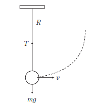
When the block is at the bottom of the circle, two forces are acting on it: Gravity (\(m g\)) pulling down and Tension (\(T\)) pulling up.
Because the block is moving in a circle, the net force must equal the centripetal force (\(F_c= \frac{m v^2}{R}\)). At the bottom, the tension has to do two jobs: cancel out gravity and provide the necessary centripetal force to keep the block from flying off in a straight line.
or \(\quad T=m g+\frac{m v^2}{R}=100+\frac{10 \times 3^2}{0.3}=400 \mathrm{~N}\)
The elongation of the wire when the block is at the bottom of the circle,
\(
\Delta L=\frac{F R}{A Y}
\)
Here, force \((F)\) is equal to the tension in the wire.
So, \(\Delta L=\frac{T R}{A Y}=\frac{400 \times 0.3}{4 \times 10^{-6} \times 2 \times 10^{11}}=1.5 \times 10^{-4} \mathrm{~m}\)

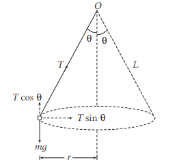
Example 6: A 2 kg mass is suspended by a rubber cord 2 m long and of cross-section \(0.5 \mathrm{~cm}^2\). It is made to describe a horizontal circle of radius \(50 \mathrm{~cm}, 4\) times in a second. Find the extension of the cord. (Take, Young’s modulus, \(Y=7 \times 10^8 \mathrm{Nm}^{-2}\) )

Solution: Given, \(m=2 \mathrm{~kg}, r=0.5 \mathrm{~m}\)
Identify the Forces:
In a horizontal circle, the horizontal component of the tension (\(T_x\)) provides the centripetal force. However, for a mass spinning this fast (4 revolutions per second), we can calculate the tension (\(T\)) required to maintain that radius (\(r\)) and angular velocity (\(\omega\)).

First, let’s find the angular velocity:
\(
\omega=2 \pi f=2 \pi \times 4=8 \pi \mathrm{rad} \mathrm{~s}^{-1}
\)
From the figure, \(T_y=T \cos \theta=m g\)
and \(F_c=T_x=T \sin \theta=\frac{m v^2}{r}=m \omega^2 r\)
Tension in cord,
\(
\begin{aligned}
T & =\sqrt{(T \sin \theta)^2+(T \cos \theta)^2} \\
& =\sqrt{\left(m \omega^2 r\right)^2+(m g)^2} \\
T & =\sqrt{\left[2 \times(8 \pi)^2 \times 0.5\right]^2+[2 \times 10]^2} \approx 631 \mathrm{~N}
\end{aligned}
\)
The extension of the cord,
\(
\begin{aligned}
\Delta L & =\frac{T L}{A Y}=\frac{631 \times 2}{0.5 \times 10^{-4} \times 7 \times 10^8} \\
& =360 \times 10^{-4} \mathrm{~m}=3.60 \mathrm{~cm}
\end{aligned}
\)

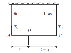
Example 7: A light rod of length \(2 m\) is suspended from the ceiling horizontally by means of two vertical wires of equal length tied to its ends. One of the wires is made of steel and is of cross-section \(10^{-3} \mathrm{~m}^2\) and the other is of brass of cross-section \(2 \times 10^{-3} \mathrm{~m}^2\). Find out the position along the rod at which a weight may be hang to produce
(i) equal stresses in both wires,
(ii) equal strains on both wires.
(Young’s modulus for steel is \(2 \times 10^{11} \mathrm{Nm}^{-2}\) and for brass is \(10^{11} \mathrm{Nm}^{-2}\))

Solution: (i) Given, \(\quad\) stress in steel \(=\) stress in brass

\(
\Rightarrow \quad \frac{T_S}{T_B}=\frac{A_S}{A_B}=\frac{10^{-3}}{2 \times 10^{-3}}=\frac{1}{2} \dots(i)
\)
As the system is in equilibrium, taking moments about \(D\), we have
\(
\begin{array}{rlrl}
& & T_S \cdot x & =T_B(2-x) \\
\therefore & \frac{T_S}{T_B} & =\frac{2-x}{x} \dots(ii)
\end{array}
\)
From Eqs. (i) and (ii), we get
\(
x=1.33 \mathrm{~m}
\)
(ii) \(\because\) Strain \(=\frac{\text { Stress }}{Y}\)
Given, strain in steel \(=\) strain in brass
\(
\begin{array}{ll}
\therefore & \frac{T_S / A_S}{Y_S}=\frac{T_B / A_B}{Y_B} \\
\therefore & \frac{T_S}{T_B}=\frac{A_S Y_S}{A_B Y_B}=\frac{\left(1 \times 10^{-3}\right)\left(2 \times 10^{11}\right)}{\left(2 \times 10^{-3}\right)\left(10^{11}\right)}=1 \dots(iii)
\end{array}
\)
From Eqs. (ii) and (iii), we have
\(
x=1 \mathrm{~m}
\)

Example 8: A steel rod of cross-sectional area \(16 \mathrm{~cm}^2\) and two brass rods each of cross-sectional area \(10 \mathrm{~cm}^2\) together support a load of \(5000 \mathrm{~kg} \mathrm{cms}^{-2}\) as shown in figure. Find the stress in the rods. (Take, Young’s modulus for steel \(=2 \times 10^6 \mathrm{~kg} \mathrm{~cm}^{-2}\) and for brass \(=1 \times 10^6 \mathrm{~kg} \mathrm{~cm}^{-2}\))

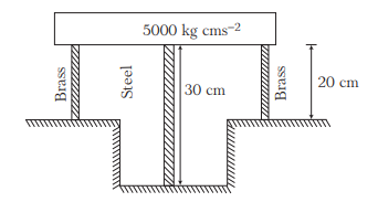
Solution: Given, area of steel rod, \(A_S=16 \mathrm{~cm}^2\)
Area of two brass rods, \(A_B=2 \times 10=20 \mathrm{~cm}^2\)
Load, \(F=5000 \mathrm{~kg} \mathrm{cms}^{-2}\)
Young’s modulus for the steel, \(Y_S=2 \times 10^6 \mathrm{~kg} \mathrm{~cm}^{-2}\)
Young’s modulus for the brass, \(Y_B=1 \times 10^6 \mathrm{~kg} \mathrm{~cm}^{-2}\)
Length of the steel rod, \(l_S=30 \mathrm{~cm}\)
Length of the brass rod, \(l_B=20 \mathrm{~cm}\)
Let \(\quad S_S=\) stress in steel and \(S_B=\) stress in brass
Decrease in length of the steel rod = Decrease in length of the brass rod
\(
\frac{S_S}{Y_S} \times l_S=\frac{S_B}{Y_B} \times l_B
\)
\(
S_S=\frac{Y_S}{Y_B} \times \frac{l_B}{l_S} \times S_B=\frac{2 \times 10^6}{1 \times 10^6} \times \frac{20}{30} \times S_B
\)
\(
\therefore \quad S_S=\frac{4}{3} S_B \dots(i)
\)
Now, using the relation,
\(
\begin{aligned}
F & =S_S A_S+S_B A_B \\
5000 & =S_S \times 16+S_B \times 20 \dots(ii)
\end{aligned}
\)
Solving Eqs. (i) and (ii), we get
\(
S_B=120.9 \mathrm{~kg} \mathrm{~cm}^{-2}
\)
∴ From Eq. (i), we get
\(
S_S=\frac{4}{3} \times 120.9=161.2 \mathrm{~kg} \mathrm{~cm}^{-2}
\)

Example 9: A copper wire of length 2.2 m and a steel wire of length 1.6 m , both of diameter 3.0 mm , are connected end to end. When stretched by a load, the net elongation is found to be 0.70 mm . Obtain the load applied.
\(
\begin{aligned}
Y_c & =1.1 \times 10^{11} \mathrm{~N} \cdot \mathrm{~m}^{-2}, \text { and } \\
Y_s & =2.0 \times 10^{11} \mathrm{~N} \cdot \mathrm{~m}^{-2} .
\end{aligned}
\)

Solution: The copper and steel wires are under a tensile stress because they have the same tension (equal to the load \(W\) ) and the same area of cross-section \(A\). We have stress \(=\) strain × Young’s modulus. Therefore
\(
W / A=Y_c \times\left(\Delta L_c / L_c\right)=Y_s \times\left(\Delta L_s / L_s\right)
\)
where the subscripts \(c\) and \(s\) refer to copper and stainless steel respectively. Or,
\(
\Delta L_c / \Delta L_s=\left(Y_s / Y_c\right) \times\left(L_c / L_s\right)
\)
Given \(L_c=2.2 \mathrm{~m}, L_s=1.6 \mathrm{~m}\),
\(
\Delta L_c / \Delta L_s=\left(2.0 \times 10^{11} / 1.1 \times 10^{11}\right) \times(2.2 / 1.6)=2.5 .
\)
The total elongation is given to be
\(
\Delta L_c+\Delta L_s=7.0 \times 10^{-4} \mathrm{~m}
\)
Solving the above equations,
\(
\Delta L_c=5.0 \times 10^{-4} \mathrm{~m}, \text { and } \Delta L_s=2.0 \times 10^{-4} \mathrm{~m} .
\)
Therefore
\(
\begin{aligned}
W & =\left(A \times Y_c \times \Delta L_c\right) / L_c \\
& =\pi\left(1.5 \times 10^{-3}\right)^2 \times\left[\left(5.0 \times 10^{-4} \times 1.1 \times 10^{11}\right) / 2.2\right] \\
& =1.8 \times 10^2 \mathrm{~N}
\end{aligned}
\)

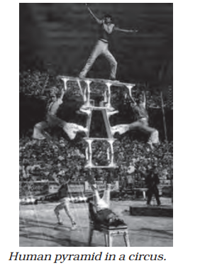
Example 10: In a human pyramid in a circus, the entire weight of the balanced group is supported by the legs of a performer who is lying on his back (as shown in Figure below). The combined mass of all the persons performing the act, and the tables, plaques etc. involved is 280 kg . The mass of the performer lying on his back at the bottom of the pyramid is 60 kg . Each thighbone (femur) of this performer has a length of 50 cm and an effective radius of 2.0 cm. Determine the amount by which each thighbone gets compressed under the extra load.

Solution: Total mass of all the performers, tables, plaques etc. \(\quad=280 \mathrm{~kg}\)
Mass of the performer \(=60 \mathrm{~kg}\)
Mass supported by the legs of the performer at the bottom of the pyramid
\(
=280-60=220 \mathrm{~kg}
\)
Weight of this supported mass
\(
=220 \mathrm{~kg} \text { wt. }=220 \times 9.8 \mathrm{~N}=2156 \mathrm{~N} .
\)
Weight supported by each thighbone of the performer \(=1 / 2(2156) \mathrm{N}=1078 \mathrm{~N}\).
The Young’s modulus for bone is given by
\(
Y=9.4 \times 10^9 \mathrm{~N} \mathrm{~m}^{-2}.
\)
Length of each thighbone \(L=0.5 \mathrm{~m}\)
the radius of thighbone \(=2.0 \mathrm{~cm}\)
Thus the cross-sectional area of the thighbone
\(
A=\pi \times\left(2 \times 10^{-2}\right)^2 \mathrm{~m}^2=1.26 \times 10^{-3} \mathrm{~m}^2 .
\)
The compression in each thighbone (\(\Delta L\)) can be computed as
\(
\begin{aligned}
\Delta L & =[(F \times L) /(Y \times A)] \\
& =\left[(1078 \times 0.5) /\left(9.4 \times 10^9 \times 1.26 \times 10^{-3}\right)\right] \\
& =4.55 \times 10^{-5} \mathrm{~m} \text { or } 4.55 \times 10^{-3} \mathrm{~cm}
\end{aligned}
\)
This is a very small change! The fractional decrease in the thighbone is \(\Delta L / L=0.000091\) or \(0.0091 \%\).

Bulk modulus of elasticity (\(B\))

When a uniform pressure (normal force) is applied all over the surface of a body, the volume of the body changes. The change in per unit volume of the body is called the volume strain and the normal force acting per unit area of the surface (pressure) is called the normal stress or volume stress. For small strains, the ratio of the volume stress to the volume strain is called the bulk modulus of the material of the body. It is denoted by \(B\), given by
\(B=\frac{\text { Volumetric Stress }}{\text { Volumetric Strain }}\)

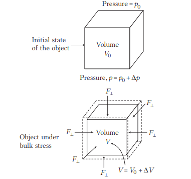
Consider a solid cube body of volume \(V\) and surface area \(A\). In order to compress the body, let a force \(F\) be applied normally on the entire surface of the body and its volume decreases by \(\Delta V\), then volumetric strain \(=-\frac{\Delta V}{V}\).
Here, negative sign shows the volume is decreasing when normal force is applied.
\(
\begin{aligned}
& \text { Stress } & =F / A \\
\therefore & B & =\frac{F / A}{-\Delta V / V} \\
\text { Then, } & B & =\frac{-p}{\Delta V / V}
\end{aligned}
\)
Here, negative sign implies that when the pressure increases, volume decreases and vice-versa. The SI unit of bulk modulus is \(\mathrm{Nm}^{-2}\) and its dimensions are \(\left[\mathrm{ML}^{-1} \mathrm{~T}^{-2}\right]\).

The relation between density \(\rho\), pressure \(\Delta p\) and bulk modulus \((B)\)

To find the relation between density and bulk modulus, we start with the definition of the Bulk Modulus (\(B\)):
\(
B=\frac{\Delta p}{-\left(\frac{\Delta V}{V}\right)}
\)
Since mass (\(m\)) is constant, we can relate volume (\(V\)) and density (\(\rho\)) using the formula \(m= \rho V\). By taking the differential of this relationship:
\(m=\rho V\)
\(0=\rho d V+V d \rho\) (since mass is constant, the change \(d m=0\))
\(\frac{d \rho}{\rho}=-\frac{d V}{V}\)
Substituting this into the Bulk Modulus formula, the relation is:
The Formula
\(
B=\rho \frac{\Delta p}{\Delta \rho}
\)
To find the Change in Density (\(\Delta \rho\)):
Simply multiply both sides by the initial density (\(\rho\)):
\(
\Delta \rho=\rho \frac{\Delta p}{B}
\)
To find the New Density (\(\rho^{\prime}\)):
The new density is the original density plus the change:
\(
\rho^{\prime}=\rho+\Delta \rho
\)
\(
\begin{aligned}
&\rho^{\prime}=\rho+\left(\rho \frac{\Delta p}{B}\right)\\
&\text { Factor out the } \rho \text { : }\\
&\rho^{\prime}=\rho\left(1+\frac{\Delta p}{B}\right)
\end{aligned}
\)

To understand why the Bulk Modulus of a gas changes depending on the thermodynamic process, we have to look at how the gas behaves under pressure in two different scenarios: when it has time to cool down (Isothermal) and when it doesn’t (Adiabatic).

Isothermal Bulk Modulus (\(B_T=P\))

In an isothermal process, the temperature remains constant (\(T=\) const). This is governed by Boyle’s Law:
\(
P V=\text { constant }
\)
To find the Bulk Modulus, we differentiate both sides with respect to volume:
\(d(P V)=0\)
\(P d V+V d P=0\)
\(V d P=-P d V\)
\(\frac{d P}{-(d V / V)}=P\)
Since the left side of that last equation is the definition of Bulk Modulus (\(B\)), we find that for an isothermal gas:
\(
B_T=P
\)
In simple terms: At a constant temperature, the gas’s resistance to being squeezed is exactly equal to the pressure it’s already under.

Adiabatic Bulk Modulus (\(B_s=\gamma P\))

In an adiabatic process, no heat enters or leaves the system (\(Q=0\)). This usually happens when a gas is compressed very quickly (like a sound wave passing through air). It follows the relation:
\(
P V^\gamma=\text { constant }
\)
(Where \(\gamma\) is the adiabatic index, the ratio of specific heats \(C_p / C_v\)).
Differentiating this:
\(d\left(P V^\gamma\right)=0\)
\(V^\gamma d P+P\left(\gamma V^{\gamma-1} d V\right)=0\)
Divide by \(V^{\gamma-1}: V d P+\gamma P d V=0\)
\(\frac{d P}{-(d V / V)}=\gamma P\)
Therefore:
\(
B_s=\gamma P
\)
In simple terms: Because the gas heats up when compressed quickly, it pushes back harder than it would if it stayed cool. This is why sound travels faster than Newton originally predicted -the air acts “stiffer” ( \(\gamma\) times stiffer) because the compressions are adiabatic.

Why is \(B=\infty\) for a Rigid Body?

Recall the formula for Bulk Modulus:
\(
B=\frac{\Delta P}{-\Delta V / V}
\)
A perfectly rigid body is defined as an object that cannot be deformed, no matter how much force you apply.
This means the change in volume (\(\Delta V\)) is always zero.
If you plug \(\Delta V=0\) into the denominator:
\(
B=\frac{\Delta P}{0}=\infty
\)
In simple terms: It would require infinite pressure to change the volume of a perfectly rigid body by even a tiny amount. In the real world, no material is perfectly rigid, but diamond or steel have very high Bulk Moduli compared to something like rubber or air.

Example 11: How much should the pressure on a litre of water be changed to compress it by \(0.10 \%\) ? (Take, bulk modulus of water \(=2.2 \times 10^9 \mathrm{~Pa}\))

Solution: Bulk modulus, \(|B|=\frac{p}{\frac{\Delta V}{V}}\)
Here, \(\frac{\Delta V}{V}=0.10 \%=\frac{0.10}{100}=1 \times 10^{-3}\)
Change in pressure,
\(
\begin{aligned}
p & =|B|\left(\frac{\Delta V}{V}\right)=\left(2.2 \times 10^9 \mathrm{~Pa}\right) \times 1 \times 10^{-3} \\
& =2.2 \times 10^6 \mathrm{~Pa}
\end{aligned}
\)

Compressibility

The reciprocal of the bulk modulus of the material of a body is called the compressibility of that material. Thus,
\(
\text { Compressibility }=\frac{1}{|B|}=\frac{\Delta V}{p V}=k
\)
The SI unit of compressibility is \(\mathrm{N}^{-1} \mathrm{~m}^2\) and its dimensions are \(\left[\mathrm{M}^{-1} \mathrm{LT}^2\right]\).
The bulk modulus is defined for all solids, liquids and gases. The value of \(B\) for solids are much larger than for liquids and that for liquids are much larger than for gases. Thus, solids are least compressible while gases are most compressible.

Example 12: What is the density of lead under a pressure of \(2 \times 10^8 \mathrm{Nm}^{-2}\), if the bulk modulus of lead is \(8 \times 10^9 \mathrm{Nm}^{-2}\) and initially the density of lead is \(11.4 \mathrm{~g} \mathrm{~cm}^{-3}\) ?

Solution: The changed density, \(\rho^{\prime}=\rho\left(1+\frac{\Delta p}{B}\right)\)
Substituting the values, we have
\(
\rho^{\prime}=11.4\left(1+\frac{2 \times 10^8}{8 \times 10^9}\right)
\)
\(
\rho^{\prime}=11.69 \mathrm{~g} \mathrm{~cm}^{-3}
\)

Example 13: The bulk modulus of water is \(2.3 \times 10^9 \mathrm{Nm}^{-2}\)
(i) Find its compressibility.
(ii) How much pressure in atmospheres is needed to compress a sample of water by \(0.1 \%\) ?

Solution: Here, \(|B|=2.3 \times 10^9 \mathrm{Nm}^{-2}\)
\(
=\frac{2.3 \times 10^9}{1.01 \times 10^5}=2.27 \times 10^4 \mathrm{~atm}
\)
(i)
\(
\begin{aligned}
\text { Compressibility } & =\frac{1}{|B|}=\frac{1}{2.27 \times 10^4} \\
& =4.4 \times 10^{-5} \mathrm{~atm}^{-1}
\end{aligned}
\)
(ii) Here, \(\frac{\Delta V}{V}=-0.1 \%=-0.001\)
∴ Required increase in pressure,
\(
\begin{aligned}
\Delta p & =B \times\left(-\frac{\Delta V}{V}\right) \\
& =2.27 \times 10^4 \times 0.001 \\
& =22.7 \mathrm{~atm}
\end{aligned}
\)

Example 14: What will be the decrease in volume of \(100 \mathrm{~cm}^3\) of water under pressure of 100 atm , if the compressibility of water is \(4 \times 10^{-5}\) per unit atmospheric pressure?

Solution: Bulk modulus, \(|B|=\frac{1}{\text { Compressibility }}=\frac{1}{k}\)
\(
\begin{aligned}
& =\frac{1}{4 \times 10^{-5}}=0.25 \times 10^5 \mathrm{~atm} \\
& =0.25 \times 10^5 \times 1.013 \times 10^5 \mathrm{Nm}^{-2} \\
& =2.533 \times 10^9 \mathrm{Nm}^{-2}
\end{aligned}
\)
Volume, \(V=100 \mathrm{~cm}^3=10^{-4} \mathrm{~m}^3\)
Pressure, \(p=100 \mathrm{~atm}=100 \times 1.013 \times 10^5 \mathrm{Nm}^{-2}\)
\(
=1.013 \times 10^7 \mathrm{Nm}^{-2}
\)
Now, apply \(\frac{1}{|B|}=k=\frac{\Delta V}{p V}\)
\(
\therefore \quad \Delta V=\frac{p V}{|B|}=\frac{1.013 \times 10^7 \times 10^{-4}}{2.533 \times 10^9}
\)
Decrease in volume,
\(
\begin{aligned}
\Delta V & \approx 0.4 \times 10^{-6} \mathrm{~m}^3 \\
& =0.4 \mathrm{~cm}^3
\end{aligned}
\)

Example 15: Find the decrease in the volume of a sample of water from the following data. Initial volume \(=2000 \mathrm{~cm}^3\), initial pressure \(=10^5 \mathrm{Nm}^{-2}\), final pressure \(=10^6 \mathrm{Nm}^{-2}\) and compressibility of water \(=25 \times 10^{-11} N^{-1} m^2\).

Solution: Bulk modulus,
\(
|B|=\frac{1}{\text { Compressibility }}=\frac{1}{25 \times 10^{-11}}=4 \times 10^9
\)
and \(|B|=\frac{-\Delta p}{\Delta V / V}\)
∴ Decrease in the volume,
\(
\begin{aligned}
\Delta V & =\frac{\Delta p V}{|B|}=\frac{\left(10^6-10^5\right)\left(2000 \times 10^{-6}\right)}{4 \times 10^9} \\
& =4.5 \times 10^{-7} \mathrm{~m}^3=4.5 \times 10^{-7} \times 10^6 \mathrm{~cm}^3 \\
& =0.45 \mathrm{~cm}^3
\end{aligned}
\)

Modulus of rigidity (Shear Modulus) (\(\eta\))

When a body is acted upon by an external force tangential to a surface of the body, where the opposite surface is kept fixed, it suffers a change in its shape but the volume remains unchanged. Then, the body is said to be sheared.

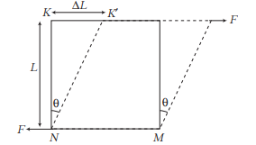
The ratio of the displacement of a layer in the direction of the tangential force to the distance of the layer from the fixed surface is called the shearing strain and the tangential force acting per unit area of the surface is called the shearing stress.
For small strain, the ratio of the shearing stress to the shearing strain is called the modulus of rigidity of the material of the body. It is denoted by \(\eta\).
Thus,
\(
\eta=\frac{F / A}{K K^{\prime} / K N}
\)
Here,
\(
\frac{K K^{\prime}}{K N}=\tan \theta \approx \theta
\)
\(
\therefore \quad \eta=\frac{F / A}{\theta}
\)
\(
\eta=\frac{F}{A \theta} \dots(i)
\)
Since, \(\theta \approx \tan \theta=\frac{K K^{\prime}}{K N}=\frac{\Delta L}{L}\)
Therefore, Eq. (i) will become
\(
\eta=\frac{F}{A} \cdot \frac{L}{\Delta L}
\)
The SI unit of modulus of rigidity is \(\mathrm{Nm}^{-2}\) and its dimensions are \(\left[\mathrm{ML}^{-1} \mathrm{~T}^{-2}\right]\).
Shear modulus (or modulus of rigidity) is generally less than Young’s modulus. For most material, \(\eta \approx Y / 3\). Shear modulus is defined for solids only.
A solid will have all the three moduli of elasticity \(Y, B\) and \(\eta\). But in case of liquid or gas only \(B\) can be defined as liquid or gas cannot be framed into a wire or no shear force can be applied on them.

Example 16: A 4 cm cube has its upper face displaced by 0.1 mm by a tangential force of 8 kN. Calculate the shear modulus of the cube.

Solution: Here, each side of the cube, \(L=4 \mathrm{~cm}\)
Area of the face over which the force is applied,
\(
A=L^2=16 \mathrm{~cm}^2
\)
Displacement, \(\Delta L=0.1 \mathrm{~mm}=0.01 \mathrm{~cm}\)
Force applied, \(F=8 \mathrm{kN}=8000 \times 10^5\) dyne
\(
=8 \times 10^8 \text { dyne }
\)
As, \(\eta=\frac{F L}{A \Delta L}\)
Shear modulus of the cube,
\(
\eta=\frac{8 \times 10^8 \times 4}{16 \times 0.01}=2 \times 10^{10} \text { dyne } / \mathrm{cm}^2
\)

Example 17: A square lead slab of side 50 cm and thickness 10.0 cm is subjected to a shearing force (on its narrow face) of magnitude \(9.0 \times 10^4 \mathrm{~N}\). The lower edge is riveted to the floor as shown in figure. How much is the upper edge is displaced, if the shear modulus of lead is \(5.6 \times 10^9 \mathrm{~Pa}\) ?

Solution: Here, \(L=50 \mathrm{~cm}=50 \times 10^{-2} \mathrm{~m}\),
\(
\eta=5.6 \times 10^9 \mathrm{~Pa}, F=9.0 \times 10^4 \mathrm{~N}
\)
Area of the face on which force is applied,
\(
A=50 \times 10 \mathrm{~cm}^2=500 \mathrm{~cm}^2=0.05 \mathrm{~m}^2
\)
If \(\Delta L\) is the displacement of the upper edge of the slab due to tangential force \(F\) applied, then
\(
\begin{gathered}
\eta=\frac{F L}{A \Delta L} \\
\Rightarrow \quad \Delta L=\frac{F L}{\eta A}=\frac{9 \times 10^4 \times 50 \times 10^{-2}}{5.6 \times 10^9 \times 0.05} \\
\Rightarrow \quad \Delta L=1.6 \times 10^{-4} \mathrm{~m}
\end{gathered}
\)

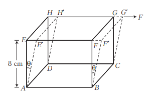
Example 18: Consider an Indian rubber cube having modulus of rigidity of \(2 \times 10^7\) dyne \(\mathrm{cm}^{-2}\) and of side 8 cm. If one side of the rubber is fixed, while a tangential force equal to the weight of 300 kg is applied to the opposite face, then find out the shearing strain produced and distance through which the strained side moves.

Solution: Given, modulus of rigidity, \(\eta=2 \times 10^7\) dyne \(\mathrm{cm}^{-2}\)

Side of the cube, \(l=8 \mathrm{~cm}\)
Area, \(A=l^2=64 \mathrm{~cm}^2\)
Force or load, \(F=300 \mathrm{kgf}=300 \times 1000 \times 981\) dyne
Modulus of rigidity, \(\eta=\frac{F}{A \theta} \Rightarrow \theta=\frac{F}{A \eta}\)
Shearing strain, \(\theta=\frac{300 \times 1000 \times 981}{64 \times 2 \times 10^7}=0.23 \mathrm{rad}\)
As, \(\eta=\frac{F}{A} \frac{l}{\Delta l} \Rightarrow \frac{\Delta l}{l}=\theta\)
Distance through which the strained side moves,
\(
\begin{array}{rlrl}
& & \Delta l & =l \theta=8 \times 0.23 \\
\Rightarrow & & \Delta l=1.84 \mathrm{~cm}
\end{array}
\)

Example 19: The average depth of Indian Ocean is about 3000 m. Calculate the fractional compression, \(\Delta V / V\), of water at the bottom of the ocean, given that the bulk modulus of water is \(2.2 \times 10^9 \mathrm{~N} \mathrm{~m}^{-2}\). (Take \(g=10 \mathrm{~m} \mathrm{~s}^{-2}\))

Solution: The pressure exerted by a 3000 m column of water on the bottom layer
\(
\begin{aligned}
p=h \rho g & =3000 \mathrm{~m} \times 1000 \mathrm{~kg} \mathrm{~m}^{-3} \times 10 \mathrm{~m} \mathrm{~s}^{-2} \\
& =3 \times 10^7 \mathrm{~kg} \mathrm{~m}^{-1} \mathrm{~s}^{-2} \\
& =3 \times 10^7 \mathrm{~N} \mathrm{~m}^{-2}
\end{aligned}
\)
Fractional compression \(\Delta V / V\), is
\(
\begin{aligned}
\Delta V / V=\text { stress } / B & =\left(3 \times 10^7 \mathrm{Nm}^{-2}\right) /\left(2.2 \times 10^9 \mathrm{Nm}^{-2}\right) \\
& =1.36 \times 10^{-2} \text { or } 1.36 \%
\end{aligned}
\)

Factors affecting elasticity

• Effect of temperature: Almost for all materials, the modulus of elasticity decreases with the rise in temperature, but the elasticity of invar remains unchanged with the change in temperature.
• Effect of impurities: The addition of impurities affects the elastic properties depending on whether impurities are themselves more or less elastic. When carbon is added to iron and potassium to gold, their elasticities are strengthened.
• Effect of annealing: By annealing (i.e. heating and then cooling gradually) large crystal grains are formed and hence, the elasticity of the material decreases.
• Effect of hammering and rolling: By hammering and rolling, crystal grains break up into smaller units and hence, the elasticity of the material increases.

Example 20: The stress-strain graph for a metallic wire is shown at two different temperatures \(T_1\) and \(T_2\), then which temperature is high \(T_1\) or \(T_2\) ?

Solution: If the slope of stress-strain curve with strain at \(X\)-axis gives the value of Young’s modulus.

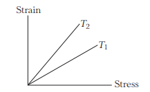
In the above graph, strain is taken along \(Y\)-axis. Therefore, the slope of graph at temperature \(T_1\) is less than the slope of graph at temperature \(T_2\).
Now, as we know with increase in temperature, the value of modulus of elasticity decreases. Therefore, temperature \(T_1\) is less than temperature \(T_2\).

Poisson’s Ratio

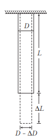
When a wire is loaded, its length increases but its diameter decreases. The strain produced in the direction of applied force is called longitudinal strain and strain produced in the perpendicular direction is called lateral strain. Within the elastic limit, the ratio of lateral strain to the longitudinal strain is called Poisson’s ratio. It is represented by (\(\sigma\)).
Let the length of the loaded wire increases from \(L\) to \(L+\Delta L\) and its diameter decreases from \(D\) to \(D-\Delta D\).
Longitudinal strain \(=\frac{\Delta L}{L}\)
Lateral strain \(=\frac{-\Delta D}{D}\)
The negative sign in the lateral strain formula \(\frac{-\Delta D}{D}\) is there to account for the inverse relationship between the change in length and the change in diameter.
\(
\begin{gathered}
\text { Poisson’s ratio is } \sigma=\frac{\text { Lateral strain }}{\text { Longitudinal strain }}=\frac{-\Delta D / D}{\Delta L / L} \\
\text { Poisson’s ratio, } \sigma=\frac{-L}{D} \cdot \frac{\Delta D}{\Delta L}
\end{gathered}
\)
The negative sign indicates that longitudinal and lateral strain are in opposite sense. It has no units and dimensions.
\(
\left\{\begin{array}{cl}
-1<\sigma<0.5, & \text { for theoretical purpose } \\
0<\sigma<0.5, & \text { for practical purpose }
\end{array}\right.
\)

Why the upper limit is 0.5?

The value \(\sigma=0.5\) represents a perfectly incompressible material. If you stretch a material with \(\sigma=0.5\), its volume remains exactly constant. Most liquids and rubbery materials sit very close to this limit (rubber is roughly 0.499). If \(\sigma\) were greater than 0.5, the material would actually decrease in volume while being pulled, which doesn’t happen in stable, isotropic solids.

Why the practical limit is \(0<\sigma<0.5\)?

For almost all common materials (metals, glass, polymers), pulling them makes them thinner.
Cork ( \(\sigma \approx 0\)): Cork is unique because when you compress it, it doesn’t bulge sideways. This is why it’s so easy to put back into a wine bottle!
Metals \((\sigma \approx 0.33)\) : Most structural metals fall in the 0.25 to 0.35 range.

Why the theoretical limit is -1?

While rare, there are “Auxetic” materials (like certain specially engineered foams or honeycombs) that have a negative Poisson’s ratio. When you stretch them, they actually get thicker.
The limit of -1 comes from the requirement that the Bulk Modulus (\(B\)) must be positive. If \(\sigma\) dropped below -1, the material would be inherently unstable-pushing on it would make it expand indefinitely.

Relation between \(Y, B, \eta\) and \(\sigma\)

There are four relations between \(Y, B, \eta\) and \(\sigma\), which can be given as follows
(1) \(B=\frac{Y}{3(1-2 \sigma)}\)
(2) \(\eta=\frac{Y}{2(1+\sigma)}\)
(3) \(\sigma=\frac{3 B-2 \eta}{2 \eta+6 B}\)
(4) \(\frac{9}{Y}=\frac{1}{B}+\frac{3}{\eta}\)

Derivation for \(B=\frac{Y}{3(1-2 \sigma)}\):

Consider a unit cube subjected to uniform tensile stress \(P\) along all three axes \((X, Y, Z)\).
Strain along X-axis:
Due to stress in \(X: \frac{P}{Y}\) (extension)
Due to stress in \(Y:-\sigma \frac{P}{\bar{Y}}\) (contraction)
Due to stress in \(Z:-\sigma \frac{P}{\bar{Y}}\) (contraction)
Total Longitudinal Strain (\(e\)) along one edge:
\(
e=\frac{P}{Y}-\sigma \frac{P}{Y}-\sigma \frac{P}{Y}=\frac{P}{Y}(1-2 \sigma)
\)
Volumetric Strain: For small strains, Volumetric Strain \(\left(\frac{\Delta V}{V}\right)\) is approximately \(3 \times\) Longitudinal Strain:
\(
\frac{\Delta V}{V}=3 e=\frac{3 P}{Y}(1-2 \sigma)
\)
Bulk Modulus (\(B\)): By definition, \(B=\frac{\text { Stress }}{\text { Volumetric Strain }}=\frac{P}{\Delta V / V}\).
\(
B=\frac{P}{\frac{3 P}{Y}(1-2 \sigma)} \Longrightarrow B=\frac{Y}{3(1-2 \sigma)}
\)
Rearranging: \(Y=3 B(1-2 \sigma)\)

Derivation of \(Y=2 \eta(1+\sigma)\)

This derivation relies on the fact that a pure shear is equivalent to a tensile stress and a compressive stress acting at right angles (\(45^{\circ}\) to the shear plane).
Let a shear stress \(\tau\) produce a shear strain \(\theta\). We know \(\eta=\frac{\tau}{\theta}\).
In a pure shear state, the linear strain along the diagonal of the cube is:
\(
\text { Strain }=\frac{\tau}{Y}(1+\sigma)
\)
From the geometry of shearing a cube, it can be proven that the linear strain along the diagonal is also equal to \(\frac{\theta}{2}\).
Equating the two:
\(
\frac{\theta}{2}=\frac{\tau}{Y}(1+\sigma)
\)
Substitute \(\theta=\frac{\tau}{\eta}\) :
\(
\frac{\tau}{2 \eta}=\frac{\tau}{Y}(1+\sigma) \Longrightarrow \frac{1}{2 \eta}=\frac{1+\sigma}{Y}
\)
Rearranging: \(Y=2 \eta(1+\sigma)\)

Deriving the “Mixed” Relations:

Once you have the two equations above, you can use basic algebra to eliminate variables:
To find \(\sigma\): Set the two expressions for \(Y\) equal to each other:
\(
3 B(1-2 \sigma)=2 \eta(1+\sigma)
\)
Solving for \(\sigma\) gives: \(\sigma=\frac{3 B-2 \eta}{6 B+2 \eta}\).
To find the relation between \(Y, B, \eta\): Eliminate \(\sigma\) by rearranging \(2 \sigma=1-\frac{Y}{3 B}\) and \(\sigma=\frac{Y}{2 \eta}-1\). Substituting these into each other and simplifying yields:
\(
\frac{9}{Y}=\frac{3}{\eta}+\frac{1}{B}
\)

Example 21: Determine the Poisson’s ratio of the material of a wire whose volume remains constant under an external normal stress.

Solution: Volume of a wire, \(V=\frac{\pi D^2}{4} l\)
As volume remains constant, the differentiation of above equation gives
\(
\begin{aligned}
0 & =\frac{\pi l}{4} \cdot 2 D \cdot d D+\frac{\pi D^2}{4} \cdot d l \\
-2 l d D & =D d l \\
\Rightarrow \quad \frac{d D}{D} & =-\frac{1}{2} \frac{d l}{l}
\end{aligned}
\)
∵ By definition, Poisson’s ratio,
\(
\sigma=\frac{-d D / D}{d l / l}=-\frac{\left(-\frac{1}{2} \frac{d l}{l}\right)}{\frac{d l}{l}}=\frac{1}{2}=0.5
\)

Example 22: A material is having Poisson’s ratio 0.2. A load is applied on it due to which it suffers the longitudinal strain \(3 \times 10^{-3}\), then find out the percentage change in its volume.

Solution: Given, Poisson’s ratio, \(\sigma=0.2\)
\(
\begin{aligned}
& \text { Longitudinal strain, } \frac{\Delta L}{L}=3 \times 10^{-3} \\
& \because \quad \text { Poisson’s ratio, } \sigma=\frac{-\Delta D / D}{\Delta L / L} \\
& \Rightarrow \quad \sigma=\frac{-\Delta R / R}{\Delta L / L} \\
& \Rightarrow \quad \frac{\Delta R}{R}=-\sigma \times \frac{\Delta L}{L}=-0.6 \times 10^{-3}
\end{aligned}
\)
\(\because \quad\) Volume, \(V=\pi R^2 L\)
Therefore, percentage change in volume,
\(
\begin{aligned}
& \left(\frac{\Delta V}{V} \times 100\right)=\left(\frac{2 \Delta R}{R}+\frac{\Delta L}{L}\right) \times 100 \\
& =\left[2 \times\left(-0.6 \times 10^{-3}\right)+3 \times 10^{-3}\right] \times 100=0.18 \%
\end{aligned}
\)

Work done or Elastic potential energy stored in a stretched wire

When you stretch a wire, you are doing work against the internal restoring forces (interatomic forces) of the material. This work is not “lost”; it is stored in the wire as Elastic Potential Energy.

Derivation: Suppose a wire of original length \(L\) and area of cross-section \(A\) is stretched by a small distance \(l\) by applying a force \(F\).
According to Young’s Modulus (\(Y\)):
\(
Y=\frac{\text { Stress }}{\text { Strain }}=\frac{F / A}{l / L} \Longrightarrow F=\frac{Y A l}{L}
\)
If we stretch the wire by an additional infinitesimal distance \(d l\), the small amount of work done \(d W\) is:
\(
d W=F \cdot d l=\left(\frac{Y A l}{L}\right) d l
\)
\(
\begin{aligned}
&\text { To find the total work done }(W) \text { in stretching the wire from } 0 \text { to a total extension } \Delta L \text { : }\\
&\begin{gathered}
W=\int_0^{\Delta L} \frac{Y A}{L} l d l=\frac{Y A}{L}\left[\frac{l^2}{2}\right]_0^{\Delta L} \\
W=\frac{1}{2} \frac{Y A(\Delta L)^2}{L}=\frac{1}{2} k(\Delta L)^2, \quad \text { where } k=\frac{Y A}{L}
\end{gathered}
\end{aligned}
\)

Standard Formulas for Elastic Potential Energy (\(U\)):

To find the energy stored, we start with the work done by a variable force. Since the force \(F\) increases linearly as the extension \(\Delta L\) increases (within the proportional limit), we use integration or the average force.
The Calculus Approach:
The work done \(W\) (which equals the potential energy \(U\)) for a small change in length \(d x\) is \(d W=F(x) d x\). Given Hooke’s Law \(F(x)=k x\), where \(k=\frac{Y A}{L}\) :
\(
U=\int_0^{\Delta L} k x d x=\left[\frac{1}{2} k x^2\right]_0^{\Delta L}=\frac{1}{2} k(\Delta L)^2
\)
The Substitution
Since \(F=k \Delta L\), we can replace one \(\Delta L\) in the equation above:
\(
\begin{gathered}
U=\frac{1}{2}(k \Delta L) \times \Delta L \\
U=\frac{1}{2} \times \text { Force × Extension }
\end{gathered}
\)
The Substitution
Since \(F=k \Delta L\), we can replace one \(\Delta L\) in the equation above:
\(
\begin{gathered}
U=\frac{1}{2}(k \Delta L) \times \Delta L \\
U=\frac{1}{2} \times \text { Force × Extension }
\end{gathered}
\)
Energy in terms of Stress and Strain:
To make this formula independent of the specific dimensions of a single wire, we can convert it into material properties (Stress and Strain).
Step 1: Start with the Force-Extension formula
\(
U=\frac{1}{2} F \Delta L
\)
Step 2: Introduce Area \((A)\) and Length \((L)\) We want to see \(\frac{F}{A}\) (Stress) and \(\frac{\Delta L}{L}\) (Strain). To do this without changing the value of the equation, we multiply the top and bottom by \(A\) and \(L\) :
\(
U=\frac{1}{2}\left(\frac{F}{A} \times A\right) \times\left(\frac{\Delta L}{L} \times L\right)
\)
Step 3: Rearrange and Group Group the terms into the definitions we recognize:
\(
U=\frac{1}{2} \times \underbrace{\left(\frac{F}{A}\right)}_{\text {Stress }} \times \underbrace{\left(\frac{\Delta L}{L}\right)}_{\text {Strain }} \times \underbrace{(A \times L)}_{\text {Volume }}
\)
\(U=\frac{1}{2} \times \text {Stress } \times \text { Strain } \times  \text { Volume }\) 

Elastic Potential Energy Density (\(u\)):

In engineering, we often care about the energy stored per unit volume of the material. This is called Energy Density.
\(
u=\frac{\text { Total Energy }}{\text { Volume }}=\frac{\frac{1}{2} \times \text { Stress } \times \text { Strain } \times V}{V}
\)
\(u=\frac{1}{2} \times \text { Stress } \times \text { Strain }\)
Using \(Y=\frac{\text { Stress }}{\text { Strain }}\), we can also write:
\(u=\frac{1}{2} \times Y \times(\text { Strain })^2\)
\(u=\frac{\text { (Stress) }^2}{2 Y}\)

Example 23: A steel wire of length 2.0 m is stretched through 2.0 mm. The cross-sectional area of the wire is \(4.0 \mathrm{~mm}^2\). Calculate the elastic potential energy stored in the wire in the stretched condition. Young modulus of steel \(=2.0 \times 10^{11} \mathrm{~N} \mathrm{~m}^{-2}\).

Solution: The strain in the wire \(\frac{\Delta l}{l}=\frac{2 \cdot 0 \mathrm{~mm}}{2 \cdot 0 \mathrm{~m}}=10^{-3}\).
The stress in the wire \(=Y \times\) strain
\(
=2.0 \times 10^{11} \mathrm{~N} \mathrm{~m}^{-2} \times 10^{-3}=2.0 \times 10^8 \mathrm{~N} \mathrm{~m}^{-2}
\)
The volume of the wire \(=\left(4 \times 10^{-6} \mathrm{~m}^2\right) \times(2.0 \mathrm{~m})\)
\(
=8.0 \times 10^{-6} \mathrm{~m}^3
\)
The elastic potential energy stored
\(
\begin{aligned}
& =\frac{1}{2} \times \text { stress × strain × volume } \\
& =\frac{1}{2} \times 2.0 \times 10^8 \mathrm{~N} \mathrm{~m}^{-2} \times 10^{-3} \times 8.0 \times 10^{-6} \mathrm{~m}^3 \\
& =0.8 \mathrm{~J}
\end{aligned}
\)

Example 24: Calculate the work done in stretching a steel wire of Young’s modulus of \(2 \times 10^{11} \mathrm{Nm}^{-2}\), length of 200 cm and area of cross-section \(0.06 \mathrm{~cm}^2\) slowly by applying a load of 40 kg without the elastic limit being reached.

Solution: Here, force, \(F=m g=40 \times 9.8 \mathrm{~N}\)
Length of wire, \(l=200 \mathrm{~cm}=2 \mathrm{~m}\)
Area of cross-section, \(A=0.06 \mathrm{~cm}^2=0.06 \times 10^{-4} \mathrm{~m}^2\)
Young’s modulus, \(Y=2 \times 10^{11} \mathrm{Nm}^{-2}\)
Work done \(=\frac{1}{2} \times\) Stretching force × Extension \(=\frac{1}{2} F \Delta l\)
\(
\begin{aligned}
& =\frac{1}{2} F \times \frac{F l}{A Y} \\
\Rightarrow \quad W & =\frac{F^2 l}{2 A Y}=\frac{(40 \times 9.8)^2 \times 2}{2 \times 0.06 \times 10^{-4} \times 2 \times 10^{11}}=0.128 \mathrm{~J}
\end{aligned}
\)

Example 25: A steel wire \(4 m\) in length is stretched through 2 mm. The cross-sectional area of the wire is \(2.0 \mathrm{~mm}^2\). If Young’s modulus of the steel is \(2 \times 10^{11} \mathrm{Nm}^{-2}\). Find
(i) the energy density of wire,
(ii) the elastic potential energy stored in the wire.

Solution: Here, length of wire, \(l=4.0 \mathrm{~m}, \Delta l=2 \times 10^{-3} \mathrm{~m}\)
Area, \(A=2.0 \times 10^{-6} \mathrm{~m}^2\)
Young’s modulus, \(Y=2.0 \times 10^{11} \mathrm{Nm}^{-2}\)
(i) The energy density of stretched wire,
\(
\begin{aligned}
u & =\frac{1}{2} \times \text { Stress × Strain }=\frac{1}{2} \times Y \times(\text { Strain })^2 \\
& =\frac{1}{2} \times 2.0 \times 10^{11} \times\left[\frac{\left(2 \times 10^{-3}\right)^2}{(4)^2}\right] \\
& =0.25 \times 10^5 \mathrm{Jm}^{-3} \\
& =2.5 \times 10^4 \mathrm{Jm}^{-3}
\end{aligned}
\)
(ii) Elastic potential energy \(=\) Energy density × Volume
\(
\begin{aligned}
& =2.5 \times 10^4 \times\left(2.0 \times 10^{-6}\right) \times 4.0 \mathrm{~J} \\
& =20 \times 10^{-2}=0.20 \mathrm{~J}
\end{aligned}
\)

Example 26: A 45 kg boy whose leg bones are \(5 \mathrm{~cm}^2\) in area and 50 cm long falls through a height of 2 m without breaking his leg bones. If the bones can stand a stress of \(0.9 \times 10^8 \mathrm{Nm}^{-2}\), then what will be the Young’s modulus for the material of the bone?

Solution: Here, mass, \(m=45 \mathrm{~kg}\), height of leg bones, \(h=2 \mathrm{~m}\)
Length, \(L=0.50 \mathrm{~m}\), area of bones, \(A=5 \times 10^{-4} \mathrm{~m}^2\)
Loss in gravitational energy = Gain in elastic energy in both leg bones
So, \(\quad m g h=2 \times\left(\frac{1}{2} \times\right.\) stress × strain × volume \()\)
Here, volume \(=A L=5 \times 10^{-4} \times 0.50=2.5 \times 10^{-4} \mathrm{~m}^3\)
\(\therefore 45 \times 10 \times 2=2 \times\left[\frac{1}{2} \times 0.9 \times 10^8 \times\right.\) strain \(\left.\times 2.5 \times 10^{-4}\right]\)
or \(\quad\) Strain \(=\frac{45 \times 10 \times 2}{0.9 \times 2.5 \times 10^4}=0.04\)
∴ Young’s modulus of bones material,
\(
\begin{aligned}
Y & =\frac{\text { Stress }}{\text { Strain }}=\frac{0.9 \times 10^8}{0.04} \\
& =2.25 \times 10^9 \mathrm{Nm}^{-2}
\end{aligned}
\)

Example 27: A rubber cord has a cross-sectional area \(1 \mathrm{~mm}^2\) and total unstretched length 10.0 cm. It is stretched to 12.5 cm and then released to project a missile of mass 5.0 g . (Take, Young’s modulus \(Y\) for rubber as \(5.0 \times 10^8 \mathrm{Nm}^{-2}\)). Calculate the velocity of projection.

Solution: Equivalent force constant of rubber cord,
\(
k=\frac{Y A}{l}=\frac{\left(5.0 \times 10^8\right)\left(1.0 \times 10^{-6}\right)}{(0.1)}=5.0 \times 10^3 \mathrm{Nm}^{-1}
\)
Now, from conservation of mechanical energy, elastic potential energy of cord = kinetic energy of missile
\(
\begin{array}{rlrl}
\therefore & \frac{1}{2} k(\Delta l)^2 =\frac{1}{2} m v^2 \\
\therefore & v =\left(\sqrt{\frac{k}{m}}\right) \Delta l=\left(\sqrt{\frac{5.0 \times 10^3}{5.0 \times 10^{-3}}}\right)(12.5-10.0) \times 10^{-2} \\
& =25 \mathrm{~ms}^{-1}
\end{array}
\)

Note: Following assumptions have been made in this example
(i) \(k\) has been assumed constant, even though it depends on the length (\(l\)).
(ii) The whole of the elastic potential energy is converting into kinetic energy of missile.

Example 28: (i) A wire 4 m long and 0.3 mm in diameter is stretched by a force of 100 N. If extension in the wire is 0.3 mm, calculate the potential energy stored in the wire.
(ii) Find the work done in stretching a wire of cross-section \(1 \mathrm{~mm}^2\) and length 2 m through 0.1 mm. Young’s modulus for the material of wire is \(2.0 \times 10^{11} \mathrm{Nm}^{-2}\).

Solution: (i) Energy stored, \(U=\frac{1}{2}\) (Stress)(Strain)(Volume)
\(
\text { or } \quad \begin{aligned}
U & =\frac{1}{2}\left(\frac{F}{A}\right)\left(\frac{\Delta l}{l}\right)(A l)=\frac{1}{2} F \cdot \Delta l \\
& =\frac{1}{2}(100)\left(0.3 \times 10^{-3}\right)=0.015 \mathrm{~J}
\end{aligned}
\)
(ii) Work done \(=\) Potential energy stored
\(
=\frac{1}{2} k(\Delta l)^2=\frac{1}{2}\left(\frac{Y A}{l}\right)(\Delta l)^2 \quad\left(\because k=\frac{Y A}{l}\right)
\)
Substituting the values, we have
\(
\begin{aligned}
W & =\frac{1}{2} \frac{\left(2.0 \times 10^{11}\right)\left(10^{-6}\right)}{(2)}\left(0.1 \times 10^{-3}\right)^2 \\
& =5.0 \times 10^{-4} \mathrm{~J}
\end{aligned}
\)

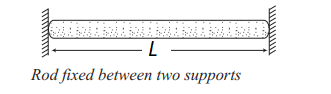
Thermal stresses and strains

When a rod is held between two rigid supports and its temperature is changed, it tries to expand or contract. Because the supports prevent this movement, internal stress is developed. Such stresses are called thermal stresses or temperature stresses. The corresponding strains are called thermal strains or temperature strains.

Thermal Strain:

If a rod of length \(L\) is free to expand, the change in length \(\Delta L\) due to a temperature change \(\Delta T\) is:
\(
\Delta L=L \alpha \Delta T
\)
(Where \(\alpha\) is the coefficient of linear expansion.)
However, Thermal Strain only occurs if the expansion is prevented. If the rod is fixed between two rigid walls, the “prevented” strain is:
\(
\text { Thermal Strain }=\frac{\Delta L}{L}=\alpha \Delta T
\)

Thermal Stress:

Using Young’s Modulus (\(Y=\frac{\text { Stress }}{\text { Strain }}\)), we can find the stress:
\(
\begin{gathered}
\text { Thermal Stress }=Y \times \text { Thermal Strain } \\
\text { Thermal Stress }=Y \alpha \Delta T
\end{gathered}
\)

Thermal Force:

The force exerted by the rod on the supports (or vice versa) is:
\(
\begin{gathered}
F=\text { Stress × Area } \\
F=Y A \alpha \Delta T
\end{gathered}
\)

Example 29: A steel wire of length 20 cm and uniform cross-section \(1 \mathrm{~mm}^2\) is tied rigidly at both the ends. If temperature of the wire is altered from \(40^{\circ} \mathrm{C}\) to \(20^{\circ} \mathrm{C}\), calculate the change in tension. (Take, coefficient of linear expansion of steel is \(1.1 \times 10^{-5}{ }^{\circ} C^{-1}\) and Young’s modulus for steel is \(2.0 \times 10^{11} \mathrm{Nm}^{-2}\))

Solution: The change in length \(l\) of the wire when wire is cooled by temperature \(\Delta t\) is given by
\(
\Delta l=l \alpha \Delta t \text { or } \Delta l / l=\alpha \Delta t \dots(i)
\)
where, \(\alpha\) is the coefficient of linear expansion. Change in the tension of the wire when it is cooled is given by
\(
\begin{aligned}
F & =Y A \Delta l / l=Y A \alpha \Delta t \quad \quad \text { [From Eq. (i)] } \\
& =\left(2.0 \times 10^{11}\right) \times\left(10^{-6}\right) \times\left(1.1 \times 10^{-5}\right) \times\left(40^{\circ}-20^{\circ}\right) \\
& =44 \mathrm{~N}
\end{aligned}
\)