8.4 Stress-strain curve

The Stress-Strain curve is a type of graph plotted between “stress and strain”. This graph explains the relationship between “stress and strain” of different materials when tensile stress is applied to them.

This curve is plotted on the basis of an experimental result. In this experiment, we take a cylinder or twine and stretch it by an applied force or tensile stress. Then we note the change in length (strain) of that body and the stress that is applied to cause the change in length. With the help of this reading, we plot a graph by taking strain along the \(x\)-axis and stress along the \(y\)-axis.

Explanation of the graph:

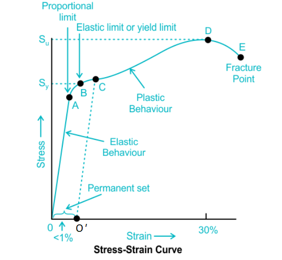
The region O To A: In the graph above, we can see that region O to A is a straight line or linear; this implies that Hooke’s law is obeyed in this region. Thus, Hooke’s law is fully obeyed in this region, the point A is known as point of proportional limit.

The region A to B: In regions A to B, the stress applied and the strain produced are not proportional to each other. When stress is increased beyond A, then for small stress, there is a large strain in the wire upto point B. So we can conclude that if the exerted force is removed, the body will return to its initial dimension.

The point B (known as the yield point): When the load is gradually removed between points O to B, the wire return to its original length. The wire regains its original dimension only when load applied is less than or equal to certain limit. This limit is called elastic limit. The point B on stress-strain curve is known as elastic limit or yield point. The material of the wire in the region OB shows the elastic behaviour, hence known as elastic region. The tensile stress corresponding to the yield point is named yield stress and denoted by \(S_y\). Further, as we increase the load, the stress starts exceeding the yield stress. This means now even if there is a small change in stress, the strain will increase rapidly.

Region B to C: If the stress or load increases beyond point B, the strain further increases. This increase in strain represented by BC part of the curve. Now, if the load is removed, the wire does not regain its original length. But the increase in the length of the wire is permanent. In other words, there is permanent strain equal to \(O O^{\prime}\) in the wire even when the stress is zero. This permanent strain in the wire is known as permanent set.

Region C to D: In this region, the strain increases very quickly even if we change the stress by a small amount. This huge increase in the strain for small stress is represented by CD part of the curve. If we withdraw the exerted force at point C between B and D, the body will not return to its initial dimension. This is a deformation produced in the body, and we call this deformation plastic deformation. At this point, the material is said to have a permanent set. The material of the wire from point C to point D shows the plastic behaviour or plastic deformation.

The point D and E: In the graph, the “D point” is called the “ultimate tensile strength of the material”. Beyond point D, additional strain is produced in the material; even if the applied tensile strength is reduced, fracture occurs. Point E is defined as a fracture point.

If the distance between point E and point D is not much, then the material is called brittle material.
If point E and point D are far apart from each other, then the material is known as ductile material.

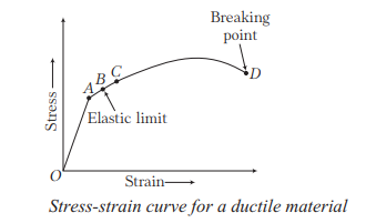
The stress-strain curve depends upon the material and varies from material to material. For example, the stress-strain curve for ductile material is different from the curve for the brittle material.

The curve shown above in figure is the stress-strain curve for a ductile material. Some examples of ductile materials are – copper, aluminium, and magnesium alloys.

Brittle material is defined as the material which shows very small elongation before reaching the fracture point.
For example – high carbon steel and concrete. The permanent elongation is less than 10% in the stress-strain curves for brittle material.

Different nature of the stress-strain curve

The stress-strain curve differ considerably for different materials. The steeper curve indicates a stiffer material, line parallel to the strain axis indicates a ductile material and in the absence of yield point or plastic behaviour refer to a brittle material.

Ductile and brittle materials

On the basis of elastic and plastic properties, materials can be classified in two ways; ductile materials and brittle materials. The materials which have large plastic range of extension are called ductile materials. As shown in the stress-strain curve, the fracture point is widely separated from the elastic limit. Such materials undergo an irreversible increase in length before snapping. So, they can be drawn into thin wires, e.g. copper, silver, iron, aluminium, etc.

The materials which have very small range of plastic extension are called brittle materials. Such materials break as soon as the stress is increased beyond the elastic limit.

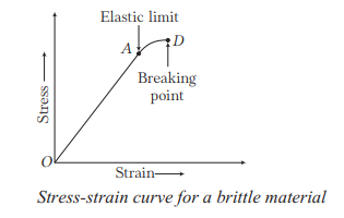
Their breaking point lies just close to their elastic limit as shown in figure, e.g. cast iron, glass, ceramics, etc.

Malleability

When a solid is compressed, a stage is reached beyond which it cannot regains its original shape after the deforming force is removed.
This is the elastic limit point \(\left(A^{\prime}\right)\) for compression. The solid then behaves like a plastic body. The yield point (\(B^{\prime}\)) obtained under compression is called crushing point.

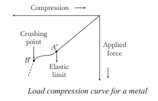
After this stage, metals are said to be malleable, i.e. they can be hammered or rolled into thin sheets, e.g. gold, silver, lead, etc.

Elastomers

The materials which can be elastically stretched to large values of strain are called elastomers. e g. . Rubber can be stretched to several times its original length but still it can regain its original length when the applied force is removed. There is no well defined plastic region, rubber just breaks when pulled beyond a certain limit. Elastic region in such cases is very large, but the material does not obey Hooke’s law.

Exception 

The figure given below represents the stress-strain curve for the elastic tissue present in the aorta, which is located in the heart. In this stress-strain curve, the elastic region is very large, but still, it doesn’t follow Hooke’s law. Also, plastic regions are absent. Such exceptions like elastic tissue in the aorta and plastic rubber are named Elastomers. They can be stretched to cause large strains.

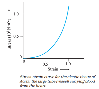
As stated earlier, the stress-strain behaviour varies from material to material. For example, rubber can be pulled to several times its original length and still returns to its original shape. Figure above shows stress-strain curve for the elastic tissue of aorta, present in the heart. Note that although elastic region is very large, the material does not obey Hooke’s law over most of the region. Secondly, there is no well defined plastic region. Substances like tissue of aorta, rubber etc. which can be stretched to cause large strains are called elastomers.

Elastic hysteresis

As a natural consequence of the elasticity after effect, the strain in the body tends to lag behind the stress applied to the body, so that during a rapidly changing stress, the strain is greater for the same value of stress. This lag of strain behind the stress is called elastic hysteresis. Due to elastic hysteresis, the original curve \((O A B)\) is not retraced when the deforming force is removed, although the body finally acquires natural length. The figure clearly indicates that the work done by the material in returning to its original shape is less than the work done by the deforming force. Hence, some amount of energy is absorbed by the material in the cycle which appears as heat.

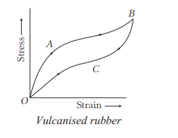
The magnitude of the energy absorbed is proportional to the area of the loop. The material having low elastic hysteresis have low elastic relaxation time.

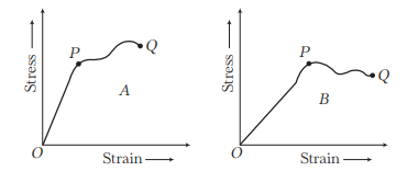
Example 30: The stress-strain graphs for two materials \(A\) and \(B\) are shown in the figure. The graphs are drawn to the same scale.

(i) Which material has a greater Young’s modulus?
(ii) Which material is more ductile?
(iii) Which material is more brittle?
(iv) Which of the two is the stronger material?

Solution: (i) Material \(A\) has a greater Young’s modulus because the slope of the linear portion of the stress-strain curve is greater for the material \(A\).
(ii) Material \(A\) is more ductile because it has a greater plastic region (from elastic limit \(P\) to breaking point \(Q\)) than material \(B\).
(iii) Material \(B\) is more brittle because it has a smaller plastic region.
(iv) Material \(A\) is stronger because it can withstand a greater stress before it breaks.