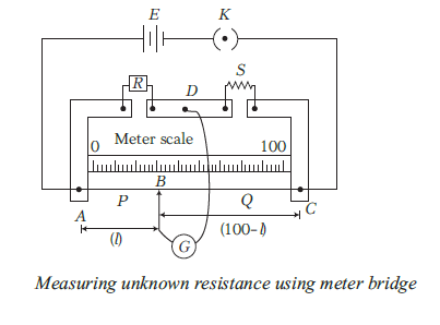
3.15 Meter Bridge

A meter bridge is a slide wire bridge or Carey Foster bridge. It is an instrument that works on the principle of the Wheatstone bridge. It consists of a straight and uniform wire along a meter scale (AC) and by varying the taping point \(B\) as shown in Fig. below, the bridge is balanced.

\(\therefore\) At balancing situation of bridge,
\(
\frac{P}{Q}=\frac{R}{S}
\)
\(
\begin{aligned}
\frac{l}{100-l} & =\frac{R}{S} \\
S & =\frac{100-l}{l} \times R
\end{aligned}
\)

Applications of meter bridge

• It is used to measure an unknown resistance by
  \(
  \text { using, } S=\frac{R(100-l)}{l}
  \)
• To compare the two unknown resistances by using,
  \(
  \frac{R}{S}=\frac{l}{100-l}
  \)

Example 88: In a meter bridge, the null point is found at a distance of 33.7 cm from A. If now a resistance of \(12 \Omega\) is connected in parallel with \(S\), the null point occurs at 51.9 cm. Determine the values of \(R\) and \(S\).

Solution: From the first balance point, we get
\(
\frac{R}{S}=\frac{33.7}{66.3} \dots(i)
\)
After \(S\) is connected in parallel with a resistance of \(12 \Omega\), the resistance across the gap changes from \(S\) to \(S_{\text {eq }}\), where
\(
S_{\text {eq }}=\frac{12 S}{S+12}
\)
and hence the new balance condition now gives
\(
\frac{51.9}{48.1}=\frac{R}{S_{\text {eq }}}=\frac{R(S+12)}{12 S} \dots(ii)
\)
Substituting the value of \(R / S\) from Eq. (i), we get
\(
\frac{51.9}{48.1}=\frac{S+12}{12} \cdot \frac{33.7}{66.3}
\)
which gives \(S=13.5 \Omega\). Using the value of \(R / S\) above, we get \(R=6.86 \Omega\).

Example 89: In the following circuit, a meter bridge is shown in its balanced state. The meter bridge wire has a resistance of \(1 \Omega- cm\). Calculate the value of the unknown resistance \(X\) and the current drawn from the battery of negligible internal resistance.

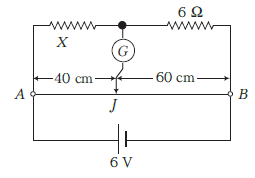
Solution:  In a balanced condition, no current flows through the galvanometer.
Here, \(P=\) resistance of wire \(A J=40 \Omega\)
\(Q=\) resistance of wire \(B J=60 \Omega\)
\(R=X, S=6 \Omega\)
In the balanced condition,
\(
\begin{gathered}
\frac{P}{Q}=\frac{R}{S} \\
\frac{40}{60}=\frac{X}{6} \\
X=4 \Omega
\end{gathered}
\)
Total resistance of wire \(A B=100 \Omega\)
Total resistance of resistances \(X\) and \(6 \Omega\) connected in series
\(
=4+6=10 \Omega
\)
This series combination is in parallel with wire \(A B\).
\(\therefore\) Equivalent resistance \(=\frac{10 \times 100}{10+100}=\frac{100}{11} \Omega\)
emf of the battery \(=6 V\)
\(\therefore\) Current drawn from the battery,
\(
I=\frac{\text { emf }}{\text { resistance }}=\frac{6}{100 / 11}=0.66 A
\)

Example 90: The given figure shows the experimental setup of a meter bridge. The null point is found to be 60 cm away from the end \(A\) with \(X\) and \(Y\) in position as shown. When a resistance of \(15 \Omega\) is connected in series with \(Y\), then the null point is found to shift by 10 cm towards the end \(A\) of the wire. Find the position of the null point, if a resistance of \(30 \Omega\) were connected in parallel with \(Y\).

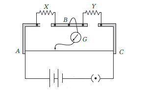
Solution: In the first case,
\(
\frac{X}{Y}=\frac{60}{40} \text { or } \frac{X}{Y}=\frac{3}{2} \dots(i)
\)
In the second case,
\(
\frac{X}{Y+15}=\frac{50}{50}=1 \dots(ii)
\)
Dividing Eq. (i) by Eq. (ii), we get
\(
\begin{gathered}
\frac{X}{Y} \times \frac{Y+15}{X}=\frac{3}{2} \times 1 \\
1+\frac{15}{Y}=\frac{3}{2} \\
Y=30 \Omega \\
X=\frac{3}{2} Y=\frac{3}{2} \times 30=45 \Omega
\end{gathered}
\)
When a resistance of \(30 \Omega\) is connected in parallel with \(Y\), then the resistance in the right gap becomes
\(
Y^{\prime}=\frac{30 Y}{30+Y}=\frac{30 \times 30}{30+30}=15 \Omega
\)
Suppose the null point occurs at \(l ~cm\) from the end \(A\).
Then,
\(
\begin{aligned}
\frac{X}{15} & =\frac{l}{100-l} \\
\frac{45}{15} & =\frac{l}{100-l} \\
300-3 l & =l \\
4 l & =300 \\
l & =75 cm
\end{aligned}
\)

Potentiometer

This is a versatile instrument. It is basically a long piece of uniform wire, sometimes a few meters in length across which a standard cell (B) is connected. In actual design, the wire is sometimes cut in several pieces placed side by side and connected at the ends by thick metal strip. (Fig. 3.28). In the figure, the wires run from \(A\) to \(C\). The small vertical portions are the thick metal strips connecting the various sections of the wire.

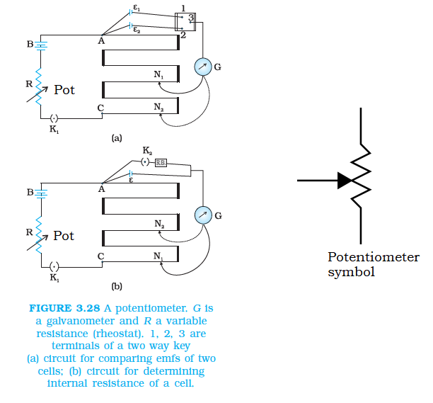
A current \(I\) flows through the wire which can be varied by a variable resistance (rheostat, \(R\) ) in the circuit. Since the wire is uniform, the potential difference between \(A\) and any point at a distance \(l\) from \(A\) is
\(
\varepsilon(l)=\phi l
\)
where \(\phi\) is the potential drop per unit length.
Figure 3.28 (a) shows an application of the potentiometer to compare the emf of two cells of emf \(\varepsilon_1\) and \(\varepsilon_2\). The points marked \(1,2,3\) form a two way key. Consider first a position of the key where 1 and 3 are connected so that the galvanometer is connected to \(\varepsilon_1\). The jockey is moved along the wire till at a point \(\mathrm{N}_1\), at a distance \(l_1\) from A , there is no deflection in the galvanometer. We can apply Kirchhoff’s loop rule to the closed loop \(\mathrm{AN}_1 \mathrm{G} 31 \mathrm{~A}\) and get,
\(
\phi l_1+0-\varepsilon_1=0 \dots(i)
\)
Similarly, if another emf \(\varepsilon_2\) is balanced against \(l_2\left(\mathrm{AN}_2\right)\)
\(
\phi l_2+0-\varepsilon_2=0 \dots(ii)
\)
From the last two equations
\(
\frac{\varepsilon_1}{\varepsilon_2}=\frac{l_1}{l_2} \dots(iii)
\)
This simple mechanism thus allows one to compare the emf’s of any two sources \(\left(\varepsilon_1, \varepsilon_2\right)\). In practice one of the cells is chosen as a standard cell whose emf is known to a high degree of accuracy. The emf of the other cell is then easily calculated from Eq. (iii).
We can also use a potentiometer to measure internal resistance of a cell [Fig. 3.28 (b)]. For this the cell (emf \(\varepsilon\) ) whose internal resistance \((r)\) is to be determined is connected across a resistance box through a key \(\mathrm{K}_2\), as shown in the figure. With key \(\mathrm{K}_2\) open, balance is obtained at length \(l_1\left(\mathrm{AN}_1\right)\). Then,
\(
\varepsilon=\phi l_1 \dots(iv)
\)
When key \(\mathrm{K}_2\) is closed, the cell sends a current (I) through the resistance box \((R)\). If \(V\) is the terminal potential difference of the cell and balance is obtained at length \(l_2\left(\mathrm{AN}_2\right)\),
\(
V=\phi l_2 \dots(v)
\)
So, we have \(\varepsilon / V=l_1 / l_2 \dots(vi)\)
But, \(\varepsilon=I(r+R)\) and \(V=I R\). This gives
\(
\varepsilon / V=(r+R) / R \dots(vii)
\)
From Eq. (vi) and (vii) we have
\(
\begin{aligned}
& (R+r) / R=l_1 / l_2 \\
& r=R\left(\frac{l_1}{l_2}-1\right) \dots(viii)
\end{aligned}
\)
Using Eq. (viii) we can find the internal resistance of a given cell.
The potentiometer has the advantage that it draws no current from the voltage source being measured. As such it is unaffected by the internal resistance of the source.

Example 91: A resistance of \(R \Omega\) draws current from a potentiometer. The potentiometer has a total resistance \(R_0 \Omega\) (F1g. 3.29). A voltage \(V\) is supplied to the potentiometer. Derive an expression for the voltage across \(R\) when the sliding contact is in the middle of the potentiometer.

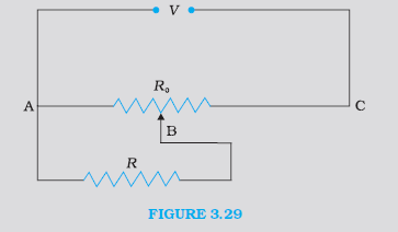
Solution: While the slide is in the middle of the potentiometer only half of its resistance \(\left(R_0 / 2\right)\) will be between the points A and B. Hence, the total resistance between A and B, say, \(R_1\), will be given by the following expression:
\(
\begin{aligned}
& \frac{1}{R_1}=\frac{1}{R}+\frac{1}{\left(R_0 / 2\right)} \\
& R_1=\frac{R_0 R}{R_0+2 R}
\end{aligned}
\)
The total resistance between A and C will be the sum of resistance between A and B and B and C, i.e., \(R_1+R_0 / 2\)
\(
\begin{aligned}
&\therefore \text { The current flowing through the potentiometer will be }\\
&I=\frac{V}{R_1+R_0 / 2}=\frac{2 V}{2 R_1+R_0}
\end{aligned}
\)
The voltage \(V_1\) taken from the potentiometer will be the product of current \(I\) and resistance \(R_1\),
\(
V_1=I R_1=\left(\frac{2 V}{2 R_1+R_0}\right) \times R_1
\)
Substituting for \(R_1\), we have a
\(
\begin{aligned}
V_1 & =\frac{2 V}{2\left(\frac{R_0 \times R}{R_0+2 R}\right)+R_0} \times \frac{R_0 \times R}{R_0+2 R} \\
V_1 & =\frac{2 V R}{2 R+R_0+2 R} \\
\text { or } \quad V_1 & =\frac{2 V R}{R_0+4 R} .
\end{aligned}
\)