Chapter-4: Motion in a plane

INTRODUCTION

In order to describe the motion of an object in two dimensions (a plane) or three dimensions (space), we need to use vectors to describe the physical quantities such as position, displacement, velocity, and acceleration. In this chapter, we study about vectors, and how to add, subtract and multiply vectors? 

SCALARS AND VECTORS

In physics, we can classify quantities as scalars or vectors. A physical quantity with only magnitude is called a scalar. It is specified completely by a single number, along with the proper unit. Examples are the distance between two points (5 meters), the mass of an object( 2 kg), and the temperature (25 °C) of a body. Scalars can be added, subtracted, multiplied, and divided just like ordinary numbers. 

A vector quantity is a quantity that has both a magnitude and a direction and obeys the triangle law of addition or equivalently the parallelogram law of addition. So, a vector is specified by giving its magnitude by a number and its direction. Some physical quantities that are represented by vectors are displacement, velocity, acceleration, and force.

The vectors are denoted by putting an arrow over the symbols representing them. Thus, we write \(\overrightarrow{A B}\), \(\overrightarrow{B C}\) etc. Sometimes a vector is represented by a single letter such as \(\vec{v}, \vec{F}\) etc. Often in  books like NCERT, the vectors are represented by bold face letters like \(\mathbf{A B}, \mathbf{B C}, \mathbf{v}, \mathbf{f}\) etc.

EQUALITY OF VECTORS

Two vectors (representing two values of the same physical quantity) are called equal if their magnitudes and directions are the same.

ADDITION OF VECTORS

If \(\vec{a}\) and \(\vec{b}\) are the two vectors to be added, a diagram is drawn in which the tail of \(\vec{b}\) coincides with the head of \(\vec{a}\). The vector joining the tail of \(\vec{a}\) with the head of \(\vec{b}\) is the vector sum of \(\vec{a}\) and \(\vec{b}\). Figure 4a shows the construction. 

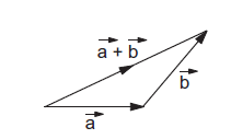figure 4a

If we draw the vectors \(\vec{a}\) and \(\vec{b}\) with both the tails coinciding (shown in figure 4b). Taking these two as the adjacent sides we complete the parallelogram. The diagonal through the common tails gives the sum of the two vectors. Thus, in figure 4b, \( \overrightarrow{A B}+\overrightarrow{A C}=\overrightarrow{A D}\).

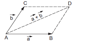figure 4b

Assume that the magnitude of \(\vec{a}=a\) and that of \(\vec{b}=b\). What is the magnitude of \(\vec{a}+\vec{b}\) and what is its direction? Suppose the angle between \(\vec{a}\) and \(\vec{b}\) is \(\theta\).We can see from figure 4c that

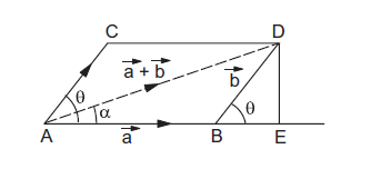figure 4c
\(
\begin{aligned}
A D^{2} &=(A B+B E)^{2}+(D E)^{2} \\
&=(a+b \cos \theta)^{2}+(b \sin \theta)^{2} \\
&=a^{2}+2 a b \cos \theta+b^{2}
\end{aligned}
\)
Thus, the magnitude of \(\vec{a}+\vec{b}\) is
\(
\sqrt{a^{2}+b^{2}+2 a b \cos \theta}
\)
Its angle with \(\vec{a}\) is \(\alpha\) where
\(
\tan \alpha=\frac{D E}{A E}=\frac{b \sin \theta}{a+b \cos \theta} .
\)

Example: 4.1

Rain is falling vertically with a speed of \(35 \mathrm{~m} \mathrm{~s}^{-1}\). Winds start blowing after some time with a speed of \(12 \mathrm{~m} \mathrm{~s}^{-1}\) in the east to west direction. In which direction should a boy waiting at a bus stop hold his umbrella?

Solution:

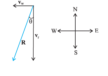figure 4d

The velocity of the rain and the wind are represented by the vectors \(\mathbf{v}_{\mathbf{r}}\) and \(\mathbf{v}_{\mathbf{w}}\) in the above figure 4d and are in the direction specified by the problem. Using the rule of vector addition, we see that the resultant of \(\mathbf{v}_{\mathbf{r}}\) and \(\mathbf{v}_{\mathbf{w}}\) is \(\mathbf{R}\) as shown in the figure. The magnitude of \(\mathbf{R}\) is
\(
R=\sqrt{v_{r}^{2}+v_{w}^{2}}=\sqrt{35^{2}+12^{2}} \mathrm{~m} \mathrm{~s}^{-1}=37 \mathrm{~m} \mathrm{~s}^{-1}
\)
The direction \(\theta\) that \(R\) makes with the vertical is given by
\(
\tan \theta=\frac{v_{w}}{v_{r}}=\frac{12}{35}=0.343
\)
Or, \(\quad \theta=\tan ^{-1}(0.343)=19^{\circ}\)
Therefore, the boy should hold his umbrella in the vertical plane at an angle of about \(19^{\circ}\) with the vertical towards the east.

MULTIPLICATION OF A VECTOR BY A REAL NUMBER

Multiplying a vector \(\vec{a}\) of magnitude \(a\) and with a positive number \(k\) gives a vector whose magnitude is changed by the factor \(k\) but the direction is the same as that of \(\vec{a}\). We define the vector \(\vec{b}=k \vec{a}\) as a vector of magnitude \(|k a|\). If \(k\) is positive the direction of the vector \(\vec{b}=k \vec{a}\) is same as that of \(\vec{a}\). If \(k\) is negative, the direction of \(\vec{b}\) is opposite to \(\vec{a}\). In particular, multiplication by \((-1\) ) just inverts the direction of the vector. The vectors \(\vec{a}\) and \(-\vec{a}\) have equal magnitudes but opposite directions. If \(\vec{a}\) is a vector of magnitude \(a\) and \(\vec{v}\) is a vector of unit magnitude in the direction of \(\vec{a}\), we can write \(\vec{a}=a \vec{v}\).

SUBTRACTION OF VECTORS

Let \(\vec{a}\) and \(\vec{b}\) be two vectors. We define \(\vec{a}-\vec{b}\) as the sum of the vector \(\vec{a}\) and the vector \((-\vec{b})\). To subtract \(\vec{b}\) from \(\vec{a}\), invert the direction of \(\vec{b}\) and add to \(\vec{a}\). Figure below shows the process.

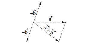figure 4e

RESOLUTION OF VECTORS

Figure 4f shows a vector \(\vec{a}=\overrightarrow{O A}\) in the \(X\)-Y plane drawn from the origin \(O\). The vector makes an angle \(\alpha\) with the \(X\)-axis and \(\beta\) with the \(Y\)-axis. Draw perpendicular \(A B\) and \(A C\) from \(A\) to the \(X\) and \(Y\) axes respectively. The length \(O B\) is called the projection of
\(\overrightarrow{O A}\) on \(X\)-axis. Similarly \(O C\) is the projection of \(\overrightarrow{O A}\) on \(Y\)-axis. According to the rules of vector addition
\(
\vec{a}=\overrightarrow{O A}=\overrightarrow{O B}+\overrightarrow{O C}
\)
Thus, we have resolved the vector \(\vec{a}\) into two parts, one along \(O X\) and the other along \(O Y\). The magnitude of the part along \(O X\) is \(O B=a \cos \alpha\) and the magnitude of the part along \(O Y\) is \(O C=a \cos \beta\). If \(\vec{i}\) and \(\vec{j}\) denote vectors of unit magnitude along \(O X\) and \(O Y\) respectively, we get
\(
\begin{aligned}
\overrightarrow{O B} &=a \cos \alpha \vec{i} \text { and } \overrightarrow{O C}=a \cos \beta \vec{j} \\
\text { so that } \quad \vec{a} &=a \cos \alpha \vec{i}+a \cos \beta \vec{j} .
\end{aligned}
\)

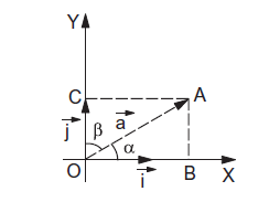Figure 4f

If the vector \(\vec{a}\) is not in the \(X-Y\) plane, it may have nonzero projections along \(X, Y, Z\) axes and we can resolve it into three parts i.e., along the \(X, Y\) and \(Z\) axes. If \(\alpha, \beta, \gamma\) be the angles made by the vector \(\vec{a}\) with the three axes respectively, we get
\(
\vec{a}=a \cos \alpha \vec{i}+a \cos \beta \vec{j}+a \cos \gamma \vec{k}
\)
where \(\vec{i}, \vec{j}\) and \(\vec{k}\) are the unit vectors along \(X, Y\) and \(Z\) axes respectively. The magnitude \((a \cos \alpha)\) is called the component of \(\vec{a}\) along \(X\)-axis, \((a \cos \beta)\) is called the component along \(Y\)-axis and \((a \cos \gamma)\) is called the component along \(Z\)-axis. In general, the component of a vector \(\vec{a}\) along a direction making an angle \(\theta\) with it is \(a \cos \theta\) (figure 4g ) which is the projection of \(\vec{a}\) along the given direction.

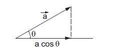Figure 4g

We can easily add two or more vectors if we know their components along the rectangular coordinate axes. Let us have
\(\begin{array}{ll}\vec{a}=a_{x} \vec{i}+a_{y} \vec{j}+a_{z} \vec{k} \\ \vec{b} =b_{x} \vec{i}+b_{y} \vec{j}+b_{z} \vec{k} \\ \text { and } \vec{c}=c_{x} \vec{i}+c_{y} \vec{j}+c_{z} \vec{k} \\ \text { then } \vec{a}+\vec{b}+\vec{c}=\left(a_{x}+b_{x}+c_{x}\right) \vec{i}+\left(a_{y}+b_{y}+c_{y}\right) \vec{j}+\left(a_{z}+b_{z}+c_{z}\right) \vec{k} .\end{array}\)
If all the vectors are in the \(X-Y\) plane then all the \(z\) components are zero and the resultant is simply
\(
\vec{a}+\vec{b}+\vec{c}=\left(a_{x}+b_{x}+c_{x}\right) \vec{i}+\left(a_{y}+b_{y}+c_{y}\right) \vec{j} .
\)
This is the sum of two mutually perpendicular vectors of magnitude \(\left(a_{x}+b_{x}+c_{x}\right)\) and \(\left(a_{y}+b_{y}+c_{y}\right)\). The resultant can easily be found to have a magnitude
\(
\sqrt{\left(a_{x}+b_{x}+c_{x}\right)^{2}+\left(a_{y}+b_{y}+c_{y}\right)^{2}}
\)
making an angle \(\alpha\) with the \(X\)-axis where
\(
\tan \alpha=\frac{a_{y}+b_{y}+c_{y}}{a_{x}+b_{x}+c_{x}} .
\)

DOT PRODUCT OR SCALAR PRODUCT OF TWO VECTORS

The dot product (also called scalar product) of two vectors \(\vec{a}\) and \(\vec{b}\) is defined as
\(
\vec{a} \cdot \vec{b}=a b \cos \theta
\)
where \(a\) and \(b\) are the magnitudes of \(\vec{a}\) and \(\vec{b}\) respectively and \(\theta\) is the angle between them. The dot product between two mutually perpendicular vectors is zero as \(\cos 90^{\circ}=0\).
The dot product is commutative and distributive.
\(
\begin{gathered}
\vec{a} \cdot \vec{b}=\vec{b} \cdot \vec{a} \\
\vec{a} \cdot(\vec{b}+\vec{c})=\vec{a} \cdot \vec{b}+\vec{a} \cdot \vec{c} .
\end{gathered}
\)

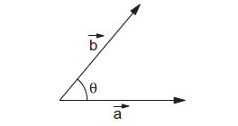Figure 4h

Dot Product of Two Vectors in terms of the Components along the Coordinate Axes

Consider two vectors \(\vec{a}\) and \(\vec{b}\) represented in terms of the unit vectors \(\vec{i}, \vec{j}, \vec{k}\) along the coordinate axes as and \(\quad \vec{b}=b_{x} \vec{i}+b_{y} \vec{j}+b_{z} \vec{k}\).
Then
\(
\begin{aligned}
\vec{a} \cdot \vec{b}=&\left(a_{x} \vec{i}+a_{y} \vec{j}+a_{z} \vec{k}\right) \cdot\left(b_{x} \vec{i}+b_{y} \vec{j}+b_{z} \vec{k}\right) \\
=& a_{x} b_{x} \vec{i} \cdot \vec{i}+a_{x} b_{y} \vec{i} \cdot \vec{j}+a_{x} b_{z} \vec{i} \cdot \vec{k} \\
&+a_{y} b_{x} \vec{j} \cdot \vec{i}+a_{y} b_{y} \vec{j} \cdot \vec{j}+a_{y} b_{z} \vec{j} \cdot \vec{k} \\
&+a_{z} b_{x} \vec{k} \cdot \vec{i}+a_{z} b_{y} \vec{k} \cdot \vec{j}+a_{z} b_{z} \vec{k} \cdot \vec{k} \ldots \quad \text { (i) }\end{aligned}
\)
Since, \(\vec{i}, \vec{j}\) and \(\vec{k}\) are mutually orthogonal,

we have \(\vec{i} \cdot \vec{j}=\vec{i} \cdot \vec{k}=\vec{j} \cdot \vec{i}=\vec{j} \cdot \vec{k}=\vec{k} \cdot \vec{i}=\vec{k} \cdot \vec{j}=0\).
Also, \(\quad \vec{i} \cdot \vec{i}=1 \times 1 \cos 0=1\).
Similarly, \(\vec{j} \cdot \vec{j}=\vec{k} \cdot \vec{k}=1\).
Using these relations in equation (i) we get
\(
\vec{a} \cdot \vec{b}=a_{x} b_{x}+a_{y} b_{y}+a_{z} b_{z}
\)

CROSS PRODUCT OR VECTOR PRODUCT OF TWO VECTORS

When two vectors are multiplied with each other and the product of the vectors is also a vector quantity, then the resultant vector is called the cross product of two vectors or the vector product. The resultant vector is perpendicular to the plane containing the two given vectors. 

The cross product or vector product of two vectors \(\vec{a}\) and \(\vec{b}\), denoted by \(\vec{a} \times \vec{b}\) is itself a vector. The magnitude of this vector is
\(
|\vec{a} \times \vec{b}|=a b \sin \theta    ——– (4.0)
\)

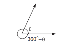Figure 4i
where \(a\) and \(b\) are the magnitudes of \(\vec{a}\) and \(\vec{b}\) respectively and \(\theta\) is the smaller angle between the two. When two vectors are drawn with both the tails coinciding, two angles are formed between them (figure 4i). One of the angles is smaller than \(180^{\circ}\) and the other is greater than \(180^{\circ}\) unless both are equal to \(180^{\circ}\). The angle \(\theta\) used in equation (4.0) is the smaller one. If both the angles are equal to \(180^{\circ}\), \(\sin \theta=\sin 180^{\circ}=0\) and hence \(|\vec{a} \times \vec{b}|=0\). Similarly if \(\theta=0, \sin \theta=0\) and \(|\vec{a} \times \vec{b}|=0\). The cross product of two parallel vectors is zero.

RIGHT-HAND RULE CROSS PRODUCT OF TWO VECTORS

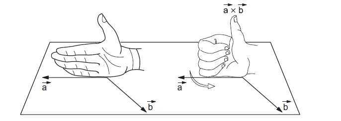Figure 4j

The direction of \(\vec{a} \times \vec{b}\) is perpendicular to both \(\vec{a}\) and \(\vec{b}\). Thus, it is perpendicular to the plane formed by \(\vec{a}\) and \(\vec{b}\). Draw the two vectors \(\vec{a}\) and \(\vec{b}\) with both the tails coinciding (figure 4j). Now place your stretched right palm perpendicular to the plane of \(\vec{a}\) and \(\vec{b}\) in such a way that the fingers are along the vector \(\vec{a}\) and when the fingers are closed they go towards \(\vec{b}\). The direction of the thumb gives direction of arrow to be put on the vector \(\vec{a} \times \vec{b}\). This is known as the right hand thumb rule.

The right-hand thumb rule makes the cross-product noncommutative. That is
\(
\vec{a} \times \vec{b}=-\vec{b} \times \vec{a} .
\)
The cross product follows the distributive law
\(
\vec{a} \times(\vec{b}+\vec{c})=\vec{a} \times \vec{b}+\vec{a} \times \vec{c} .
\)
It does not follow the associative law
\(
\vec{a} \times(\vec{b} \times \vec{c}) \neq(\vec{a} \times \vec{b}) \times \vec{c} .
\)
When we choose a coordinate system any two perpendicular lines may be chosen as \(X\) and \(Y\) axes. However, once \(X\) and \(Y\) axes are chosen, there are two possible choices of \(Z\)-axis. The \(Z\)-axis must be perpendicular to the \(X-Y\) plane. But the positive direction of \(Z\)-axis may be defined in two ways. We choose the positive direction of \(Z\)-axis in such a way that
\(
\vec{i} \times \vec{j}=\vec{k} .
\)
Such a coordinate system is called a right-handed system. In such a system
\(
\vec{j} \times \vec{k}=\vec{i} \quad \text { and } \vec{k} \times \vec{i}=\vec{j} .
\)
Of course \(\vec{i} \times \vec{i}=\vec{j} \times \vec{j}=\vec{k} \times \vec{k}=0\).

Example: 4.2

The vector \(\vec{A}\) has a magnitude of 5 unit, \(\vec{B}\) has a magnitude of 6 unit, and the cross product of \(\vec{A}\) and \(\vec{B}\) has a magnitude of 15 unit. Find the angle between \(\vec{A}\) and \(\vec{B}\).
Solution: If the angle between \(\vec{A}\) and \(\vec{B}\) is \(\theta\), the cross product will have a magnitude
\(
|\vec{A} \times \vec{B}|=A B \sin \theta
\)
\(
15=5 \times 6 \sin \theta
\)
\(
\sin \theta=\frac{1}{2} \text {. }
\)
Thus, \(\theta=30^{\circ} \text { or, } 150^{\circ}.\)

Cross Product of Two Vectors in terms of the Components along the Coordinate Axes

Let \(\quad \vec{a}=a_{x} \vec{i}+a_{y} \vec{j}+a_{z} \vec{k}\) and
\(
\vec{b}=b_{x} \vec{i}+b_{y} \vec{j}+b_{z} \vec{k}
\)

Then \(\vec{a} \times \vec{b}=\left(a_{x} \vec{i}+a_{y} \vec{j}+a_{z} \vec{k}\right) \times\left(b_{x} \vec{i}+b_{y} \vec{j}+b_{z} \vec{k}\right)\)
\(
\begin{aligned}
=& a_{x} b_{x} \vec{i} \times \vec{i}+a_{x} b_{y} \vec{i} \times \vec{j}+a_{x} b_{z} \vec{i} \times \vec{k} \\
&+a_{y} b_{x} \vec{j} \times \vec{i}+a_{y} b_{y} \vec{j} \times \vec{j}+a_{y} b_{z} \vec{j} \times \vec{k} \\
&+a_{z} b_{x} \vec{k} \times \vec{i}+a_{z} b_{y} \vec{k} \times \vec{j}+a_{z} b_{z} \vec{k} \times \vec{k} \\
=& a_{x} b_{y} \vec{k}+a_{x} b_{z}(-\vec{j})+a_{y} b_{x}(-\vec{k})+a_{y} b_{z}(\vec{i}) \\
&+a_{z} b_{x}(\vec{j})+a_{z} b_{y}(-\vec{i}) \\
=&\left(a_{y} b_{z}-a_{z} b_{y}\right) \vec{i}+\left(a_{z} b_{x}-a_{x} b_{z}\right) \vec{j} \\
&+\left(a_{x} b_{y}-a_{y} b_{x}\right) \vec{k} .
\end{aligned}
\)

Zero Vector

A null or zero vector is a vector with zero magnitude. Since the magnitude is zero, we don’t have to specify its direction. The direction of a zero vector is indeterminate. We can write this vector as \(\overrightarrow{0}\). The concept of a zero vector is also helpful when we consider the vector product of parallel vectors. If \(\vec{A} \| \vec{B}\), the vector \(\vec{A} \times \vec{B}\) is zero vector. For any vector \(\vec{A}\)
\(
\begin{aligned}
&\vec{A}+\overrightarrow{0}=\vec{A} \\
&\vec{A} \times \overrightarrow{0}=\overrightarrow{0}
\end{aligned}
\)
and for any number \(\lambda\),
\(
\lambda \overrightarrow{0}=\overrightarrow{0} .
\)

ELEMENTS OF CALCULUS

1. Differential Calculus
2. Integral Calculus

Differential Calculus: \(\frac{d y}{d x}\)

Using the concept of ‘differentlal coefflcient’ or ‘derivative’, we can easily define velocity and acceleration. Suppose we have a quantity \(y\) whose value depends upon a single variable \(x\), and is expressed by an equation defining \(y\) as some specific function of \(x\). This is represented as:
\(
y=f(x)
\)
This relationship can be visualised by drawing a graph of function \(y=f(x)\) regarding \(y\) and \(x\) as Cartesian coordinates, as shown in Figure 4k.

 

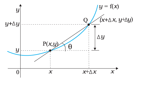Figure 4k

Consider the point \(\mathrm{P}\) on the curve \(y=f(x)\) whose coordinates are \((x, y)\) and another point \(\mathrm{Q}\) where coordinates are \((x+\Delta x, y+\Delta y)\). The slope of the line joining \(\mathrm{P}\) and \(\mathrm{Q}\) is given by:

\(
\tan \theta=\frac{\Delta y}{\Delta x}=\frac{(y+\Delta y)-y}{\Delta x}
\)

Suppose now that the point \(Q\) moves along the curve towards \(P\). In this process, \(\Delta y\) and \(\Delta x\) decrease and approach zero; though their ratio \(\frac{\Delta y}{\Delta x}\) will not necessarily vanish. What happens to the line PQ as \(\Delta y \rightarrow 0, \Delta x \rightarrow 0\). You can see that this line becomes a tangent to the curve at point P. This means that \(\tan \theta\) approaches the slope of the tangent at \(\mathrm{P}\), denoted by \(m\):

\(
m=\lim _{\Delta x \rightarrow 0} \frac{\Delta y}{\Delta x}=\lim _{\Delta x \rightarrow 0} \frac{(y+\Delta y)-y}{\Delta x}
\)

The limit of the ratio \(\Delta y / \Delta x\) as \(\Delta x\) approaches zero is called the derivative of \(y\) with respect to \(x\) and is written as \(\mathrm{d} y / \mathrm{d} x\). It represents the slope of the tangent line to the curve \(y=f(x)\) at the point \((x, y)\).
Since \(y=f(x)\) and \(y+\Delta y=f(x+\Delta x)\), we can write the definition of the derivative as:

\(
\frac{\mathrm{dy}}{\mathrm{dx}}=\frac{\mathrm{d} f(x)}{\mathrm{dx}}=\lim _{\Delta \mathrm{x} \rightarrow 0} \frac{\Delta y}{\Delta x}=\lim _{\Delta x \rightarrow 0}\left[\frac{f(x+\Delta x)-f(x)}{\Delta x}\right]
\)

VELOCITY AND ACCELERATION

The velocity (instantaneous velocity) is given by the limiting value of the average velocity as the time interval approaches zero:

\(v=\lim _{\Delta t \rightarrow 0} \frac{\Delta x}{\Delta t}=\frac{\mathrm{d} x}{\mathrm{~d} t}\)

The acceleration (instantaneous acceleration) is the limiting value of the average acceleration as the time interval approaches zero:

\(a=\lim _{\Delta t \rightarrow 0} \frac{\Delta v}{\Delta t}=\frac{\mathrm{d} v}{\mathrm{~d} t}=\frac{\mathrm{d}^{2} x}{\mathrm{~d} t^{2}}\)

POINTS TO REMEMBER:

\(\frac{d y}{d x}\) for some common functions

y	\(\frac{d y}{d x}\)
\(x^{n}\)	\(n x^{n-1}\)
\(\ln x\)	\(\frac{1}{x}\)
\(e^{x}\)	\(e^{x}\)
\(\sin x\)	\(\cos x\)
\(\cos x\)	\(-\sin x\)
\(\tan x\)	\(\sec ^{2} x\)
\(\cot x\)	\(-\operatorname{cosec}^{2} x\)
\(\sec x\)	\(\sec x \tan x\)
\(\operatorname{cosec} x\)	\(-\operatorname{cosec} x \cot x\)
\(\frac{d}{d x}(a y)\)	\(a \frac{d y}{d x}\)
\(\frac{d}{d x}(u+v)\)	\(\frac{d u}{d x}+\frac{d v}{d x}\)
\(\frac{d}{d x}(u v)\)	\(u \frac{d v}{d x}+v \frac{d u}{d x}\)
\(\frac{d}{d x}\left(\frac{u}{v}\right)\)	\(\frac{v \frac{d u}{d x}-u \frac{d v}{d x}}{v^{2}}\)
\(\frac{d y}{d x}\)	\(\frac{d y}{d u} \cdot \frac{d u}{d x}\)

Example: 4.3

Find \(\frac{d y}{d x}\) if \(y=e^{x} \sin x\)

Solution: \(y=e^{x} \sin x\).
\(
\begin{aligned}
\frac{d y}{d x} &=\frac{d}{d x}\left(e^{x} \sin x\right)=e^{x} \frac{d}{d x}(\sin x)+\sin x \frac{d}{d x}\left(e^{x}\right) \\
&=e^{x} \cos x+e^{x} \sin x=e^{x}(\cos x+\sin x)
\end{aligned}
\)

MAXIMA AND MINIMA

One of the great powers of calculus is in the determination of the maximum or minimum value of a function. 

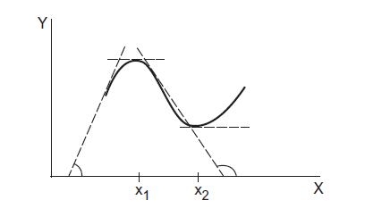Figure 4l

Assume a quantity \(y\) depends on another quantity \(x\) in a manner shown in figure 4l. It becomes maximum at \(x_{1}\) and minimum at \(x_{2}\).

Just before the maximum, the slope is positive, at the maximum, it is zero and just after the maximum, it is negative. Thus, \(\frac{d y}{d x}\) decreases at a maximum, and hence the rate of change of \(\frac{d y}{d x}\) is negative at a maximum i.e.
\(
\frac{d}{d x}\left(\frac{d y}{d x}\right)<0 \text { at a maximum. }
\)
The quantity \(\frac{d}{d x}\left(\frac{d y}{d x}\right)\) is the rate of change of the slope. It is written as \(\frac{d^{2} y}{d x^{2}}\).

Thus, the condition of a maximum is
\(\begin{aligned}
&\frac{d y}{d x}=0 \\
&\frac{d^{2} y}{d x^{2}}<0
\end{aligned}\)

Similarly, at a minimum the slope changes from negative to positive. The slope increases at such a point and hence \(\frac{d}{d x}\left(\frac{d y}{d x}\right)>0\).

The condition of a minimum is 

\(\begin{aligned}
&\frac{d y}{d x}=0 \\
&\frac{d^{2} y}{d x^{2}}>0
\end{aligned}\)

Example: 4.4

The height reached in time \(t\) by a particle thrown upward with a speed \(u\) is given by
\(
h=u t-\frac{1}{2} g t^{2}
\)
where \(g=9.8 \mathrm{~m} / \mathrm{s}^{2}\) is a constant. Find the time taken in reaching the maximum height.

Solution: The height \(h\) is a function of time. Thus, \(h\) will be maximum when \(\frac{d h}{d t}=0\). We have,
\(
\begin{aligned}
h &=u t-\frac{1}{2} g t^{2} \\
\frac{d h}{d t} &=\frac{d}{d t}(u t)-\frac{d}{d t}\left(\frac{1}{2} g t^{2}\right)
\end{aligned}
\)

\(\begin{aligned}
&=u \frac{d t}{d t}-\frac{1}{2} g \frac{d}{d t}\left(t^{2}\right) \\
&=u-\frac{1}{2} g(2 t)=u-g t
\end{aligned}
\)
For maximum \(h\),
\(
\frac{d h}{d t}=0
\)
or, \(u-g t=0 \quad\) or, \(\quad t=\frac{u}{g} .\)

INTEGRAL CALCULUS

Integral is the representation of the area of a region under a curve. Let us take the example shown in Figure 4m. Suppose a variable force \(F(x)\) acts on a particle in its motion along \(x\) – axis from \(x=\) a to \(x=b\). The problem is to determine the work done \((W)\) by the force on the particle during the motion. 

Figure 4m shows the variation of \(F(x)\) with \(x\). If the force were constant, work would be simply the area \(F(b-a)\) as shown in Figure 4m. But in the general case, force is varying.

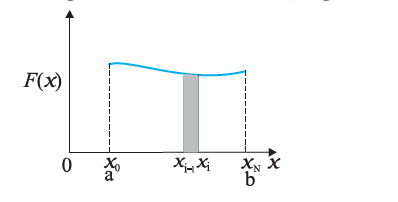Figure 4m

To calculate the area under this curve(Figure 4m), let us employ the following trick. Divide the interval on \(x\)-axis from \(a\) to \(b\) into a large number \((N)\) of small intervals: \(x_{0}(=a)\) to \(x_{1}, x_{1}\) to \(x_{2} , x_{2}\) to \(x_{3}\), \(x_{N-1}\) to \(x_{N}(=b)\). The area under the curve is thus divided into \(N\) strips. Each strip is approximately a rectangle, since the varlation of \(F(x)\) over a strip is negligible. The area of the \(i^{\text {th }}\) strip shown [Figure 4m] is then approximately
\(
\Delta A_{i}=F\left(x_{i}\right)\left(x_{i}-x_{i-1}\right)=F\left(x_{i}\right) \Delta x
\)
where \(\Delta x\) is the width of the strip which we have taken to be the same for all the strips. You may wonder whether we should put \(F\left(x_{i-1}\right)\) or the mean of \(F\left(x_{i}\right)\) and \(F\left(x_{i-1}\right)\) in the above expression. If we take \(N\) to be very very large \((N \rightarrow \infty)\), it does not really matter, since then the strip will be so thin that the difference between \(F\left(x_{i}\right)\) and \(F\left(x_{i-1}\right)\) is vanishingly small. The total area under the curve then is:
\(
A=\sum_{i=1}^{N} \Delta A_{i}=\sum_{i=1}^{N} F\left(x_{i}\right) \Delta x
\)
The limit of this sum as \(N \rightarrow \infty\) is known as the integral of \(F(x)\) over \(x\) from a to b. It is given a special symbol as shown below:
\(
A=\int_{a}^{b} F(x) d x
\)

Indefinite Integral

An indefinite integral is a function that takes the antiderivative of another function. A most significant mathematical fact is that integration is, in a sense, an inverse of differentiation.
Suppose we have a function \(g(x)\) whose derivative is \(f(x)\), i.e. \(f(x)=\frac{d g(x)}{d x}\)
The function \(g(x)\) is known as the indefinite integral of \(f(x)\) and is denoted as:
\(
g(x)=\int f(x) d x
\)

Definite IntegralAn integral with lower and upper limits is known as a definite integral. It is a number. Indefinite integral has no limits; it is a function. A fundamental theorem of mathematics states that
\(
\int_{a}^{b} f(x) d x=\left.g(x)\right|_{a} ^{b} \equiv g(b)-g(a)
\)

Integration Formulae:

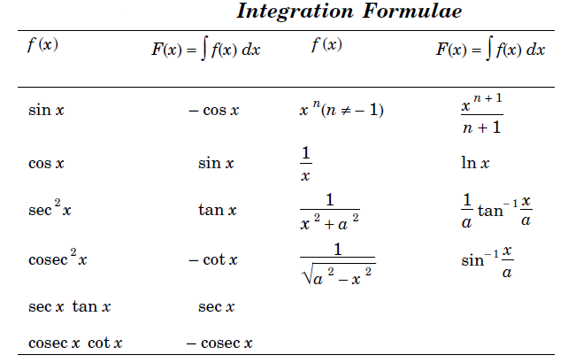
Some useful rules for integration are as follows:
(1) \(\int c f(x) d x=c \int f(x) d x\) where \(c\) is a constant

(2) \(Let \int f(x) d x=F(x)\) then \(\int f(c x) d x=\frac{1}{c} F(c x) .\)

(3) \(\int[f(x)+g(x)] d x=\int f(x) d x+\int g(x) d x\).

RELATIVE VELOCITY IN TWO DIMENSIONS

The concept of relative velocity can be easily extended to include motion in a plane or in three dimensions. Suppose that two objects A and B are moving with velocities \(\mathbf{v}_{\mathbf{A}}\) and \(\mathbf{v}_{\mathbf{B}}\) (each with respect to some common frame of reference, say ground.). Then, the velocity of object A relative to that of B is:
\(
\mathbf{v}_{\mathrm{AB}}=\mathbf{v}_{\mathrm{A}}-\mathbf{v}_{\mathrm{B}}
\)
and similarly, the velocity of object B relative to that of $\mathrm{A}$ is :
\(
\mathbf{v}_{B A}=\mathbf{v}_{B}-\mathbf{v}_{\mathrm{A}}
\)
Therefore, \(\mathbf{v}_{\mathrm{AB}}=-\mathbf{v}_{\mathrm{BA}}\)
and, \(\left|\mathbf{v}_{\mathrm{AB}}\right|=\left|\mathbf{v}_{\mathrm{BA}}\right|\)

MOTION IN A PLANE WITH CONSTANT ACCELERATION

Suppose that an object is moving in \(x-y\) plane and its acceleration a is constant. Over an interval of time, the average acceleration will equal this constant value. Now, let the velocity of the object be \(\mathbf{v}_{0}\) at time \(t=0\) and \(\mathbf{v}\) at time \(t\). Then, by definition
\(\quad \mathbf{a}=\frac{\mathbf{v}-\mathbf{v}_{0}}{t-0}=\frac{\mathbf{v}-\mathbf{v}_{0}}{t}\) Or, \(\mathbf{v}=\mathbf{v}_{\mathbf{0}} {+} \mathbf{a} t\), In terms of components : 

\(v_{x}=v_{o x}+a_{x} t \) \(, v_{y}=v_{o y}+a_{y} t \)
Let us now find how the position \(\mathbf{r}\) changes with time. We follow the method used in the one-dimensional case. Let \(\mathbf{r}_{\mathrm{o}}\) and \(\mathbf{r}\) be the position vectors of the particle at time 0 and \(t\) and let the velocitles at these instants be \(\mathbf{v}_{\mathbf{o}}\) and \(\mathbf{v}\). Then, over this time interval \(t\), the average velocity is \(\left(\mathbf{v}_{0}+\mathbf{v}\right) / 2\). The displacement is the average velocity multiplied by the time interval: 

\(\mathbf{r}-\mathbf{r}_{0}=\left(\frac{\mathbf{v}+\mathbf{v}_{0}}{2}\right) t=\left(\frac{\left(\mathbf{v}_{0}+\mathbf{a} t\right)+\mathbf{v}_{0}}{2}\right) t\)

\(
=\mathbf{v}_{0} t+\frac{1}{2} \mathbf{a} t^{2}
\)
Or, \(\quad \mathbf{r}=\mathbf{r}_{\mathbf{0}}+\mathbf{v}_{0} t+\frac{1}{2} \mathbf{a} t^{2}\)
Above Equation can be written in component form as
\(
\begin{aligned}
&x=x_{0}+v_{o x} t+\frac{1}{2} a_{x} t^{2} \\
&y=y_{0}+v_{o y} t+\frac{1}{2} a_{y} t^{2}
\end{aligned}
\)

Note: The velocity of the object \(\mathbf{v}_{0}\) at time \({t=0}\) is referred as \({u}\) in many reference physics books.

PROJECTILE MOTION

When a particle is thrown obliquely near the earth’s surface, it moves along a curved path. Such a particle is called a projectile and its motion is called projectile motion. If we neglect the air resistance the acceleration of a particle is then almost constant. It is in the vertically downward direction and its magnitude is \(g\) which is about \(9.8 \mathrm{~m} / \mathrm{s}^{2}\).

Figure 4n shows a particle projected from the point \(O\) with an initial velocity \(u\) at an angle \(\theta\) with the horizontal. It goes through the highest point \(A\) and falls at \(B\) on the horizontal surface through \(O\). The point \(O\) is called the point of projection, the angle \(\theta\) is called the angle of projection, and the distance \(O B\) is called the horizontal range or simply range. The total time taken by the particle in describing the path \(O A B\) is called the time of flight.

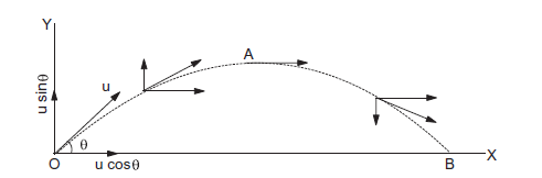Figure 4n

The motion of the projectile can be discussed separately for the horizontal and vertical parts. We take the origin at the point of projection. The instant when the particle is projected is taken as \(t=0\). The plane of motion is taken as the \(X-Y\) plane. The horizontal line \(O X\) is taken as the \(X\)-axis and the vertical line \(O Y\) as the \(Y\)-axis. Vertically upward direction is taken as the positive direction of the \(Y\)-axis. After the object has been projected, the acceleration acting on it is due to gravity which is directed vertically downward.
The components of initial velocity \({u}\) and acceleration \({a}\) are: 

\(\quad u_{x}=u \cos \theta ; \quad a_{x}=0\\\)\(\quad u_{y}=u \sin \theta ; \quad a_{y}=-g .\)

Horizontal Motion
As \(a_{x}=0\), we have \(v_{x}=u_{x}+a_{x} t=u_{x}=u \cos \theta\)

and \(x=u_{x} t+\frac{1}{2} a_{x} t^{2}=u_{x} t=u t \cos \theta .\)
As indicated in figure 4n, the \(x\)-component of the velocity remains constant as the particle moves.

Vertical Motion

The acceleration of the particle is \(g\) in the downward direction. Thus, \(a_{y}=-g\). The \(y\)-component of the initial velocity is \(u_{y}\). Thus,
\(
\begin{aligned}
v_{y} &=u_{y}-g t = u \sin \theta -g t \\
y &=u_{y} t-\frac{1}{2} g t^{2} .
\end{aligned}
\)
Also we have,
\(
v_{y}^{2}=u_{y}^{2}-2 g y .
\)

The vertical motion is identical to the motion of a particle projected vertically upward with speed \(u \sin \theta\). The horizontal motion of the particle is identical to a particle moving horizontally with uniform velocity \(u \cos \theta\).

Equation of path of a projectile
What is the shape of the path followed by the projectile? This can be seen by eliminating the time between the expressions for \(x\) and \(y\) as given in the two equations below derived earlier.

\(\begin{aligned}x=u t \cos \theta; y=u t \sin \theta-\frac{1}{2} g t^{2} \end{aligned}\)

We obtain: \(
y=\left(\tan \theta\right) x-\frac{g}{2\left(u \cos \theta\right)^{2}} x^{2}
\)
Now, since \(g, \theta\) and \(u\) are constants, above equation is of the form \(y=a x+b x^{2}\), in which \(a\) and \(b\) are constants. This is the equation of a parabola, i.e. the path of the projectile is a parabola.

Time of Flight
In Figure 4n, the particle is projected from the point \(O\) and reaches the same horizontal plane at the point \(B\). The total time taken to reach \(B\) is the time of flight.

Suppose the particle is at \(B\) at a time \(t\). The equation for horizontal motion gives
\(
O B=x=u t \cos \theta
\)
The \(y\)-coordinate at the point \(B\) is zero. Thus, from the equation of vertical motion,
\(
y=u t \sin \theta-\frac{1}{2} g t^{2}
\)
or, \(\quad 0=u t \sin \theta-\frac{1}{2} g t^{2}\)
or, \(\quad t\left(u \sin \theta-\frac{1}{2} g t\right)=0 .\)
Thus, either \(t=0\) or, \(t=\frac{2 u \sin \theta}{g}\).
Now \(t=0\) corresponds to the position \(O\) of the particle. The time at which it reaches \(B\) is thus,
\(
T_{f}=\frac{2 u \sin \theta}{g}
\)
We call \(T_{f}\) the time of flight of the projectile. 

Time of maximum height
How much time does the projectile take to reach the maximum height? Let this time be denoted by \(t_{m^{*}}\) Since at this point, \(v_{y}=0\), we have:
\(\quad \begin{aligned} v_{y}=u \sin \theta-g t_{m}=0 \\
\text { Therefore },  t_{m}={u} \sin \theta / g
\end{aligned}
\)

We note that \(T_{f}=2 t_{m}\), which is expected because of the symmetry of the parabolic path.

Maximum height of a projectile
The maximum height \(h_{m}\) reached by the projectile can be calculated by substituting \(t=t_{m}\) in the equation \(y=u t \sin \theta-\frac{1}{2} g t^{2}\).

\(\begin{aligned}
&=(u \sin \theta)\left(\frac{u \sin \theta}{g}\right)-\frac{1}{2} g\left(\frac{u \sin \theta}{g}\right)^{2} \\
&=\frac{u^{2} \sin ^{2} \theta}{g}-\frac{1}{2} \frac{u^{2} \sin ^{2} \theta}{g} \\
&=\frac{u^{2} \sin ^{2} \theta}{2 g}
\end{aligned}\)

Example: 4.5

A ball is thrown from a field with a speed of \(12.0 \mathrm{~m} / \mathrm{s}\) at an angle of \(45^{\circ}\) with the horizontal. At what distance will it hit the field again? Take \(g=10.0 \mathrm{~m} / \mathrm{s}^{2}\).

Solution: The horizontal range \(=\frac{u^{2} \sin 2 \theta}{g}\)
\(
\begin{aligned}
&=\frac{(12 \mathrm{~m} / \mathrm{s})^{2} \times \sin \left(2 \times 45^{\circ}\right)}{10 \mathrm{~m} / \mathrm{s}^{2}} \\
&=\frac{144 \mathrm{~m} / \mathrm{s}^{2}}{10.0 \mathrm{~m} / \mathrm{s}^{2}}=14.4 \mathrm{~m} .
\end{aligned}
\)
Thus, the ball hits the field at \(14.4 \mathrm{~m}\) from the point of projection.

Horizontal range of a projectile
The horizontal distance travelled by a projectile from its initial position \((x=y=0)\) to the position where it passes \(y=0\) during its fall is called the horizontal range, \(R\). It is the distance travelled during the time of flight \(T_{f}\). Therefore, the range \(R\) can be calculated (which is the distance \(O B\) as shown in Figure 4n). by using the distance travelled by the particle in time \(T_{f}=\frac{2 u \sin \theta}{g}\) in the equation of horizontal motion as shown below:
\(
\begin{aligned}
x &=(u \cos \theta) t \\
\text { or, } \quad R &=(u \cos \theta) T_{f} =(u \cos \theta)\left(\frac{2 u \sin \theta}{g}\right) \\
&=\frac{2 u^{2} \sin \theta \cos \theta}{g} \\
&=\frac{u^{2} \sin 2 \theta}{g}
\end{aligned}
\)

The range equation R shows that for a given projection velocity \(u, R\) is maximum when \(\sin\) \(2 \theta\) is maximum, i.e., when \(\theta_{0}=45^{\circ}\). The maximum horizontal range is, therefore,
\(
R_{m}=\frac{u^{2}}{g}
\)

Example: 4.6

A hiker stands on the edge of a cliff \(490 \mathrm{~m}\) above the ground and throws a stone horizontally with an initial speed of \(15 \mathrm{~m} \mathrm{~s}^{-1}\). Neglecting air resistance, find the time taken by the stone to reach the ground, and the speed with which it hits the ground. (Take \(g=9.8 \mathrm{~m} \mathrm{~s}^{-2}\) ).

Solution:  We choose the origin of the \(x\)-, and \(y\)– axis at the edge of the cliff and \(t=0 \mathrm{~s}\) at the instant the stone is thrown. Choose the positive direction of \(x\)-axis to be along the initial velocity and the positive direction of \(y\)-axis to be the vertically upward direction. The \(x\)-, and \(y\)– components of the motion can be treated independently. The equations of motion are:
\(x(t)=x_{o}+v_{0 x} t\)
\(y(t)=y_{o}+v_{\text {oy }} t+(1 / 2) a_{y} t^{2}\)
Here, \(x_{0}=y_{0}=0, v_{\text {oy }}=0, a_{y}=-g=-9.8 \mathrm{~m} \mathrm{~s}^{-2}\), \(v_{\mathrm{ox}}=15 \mathrm{~m} \mathrm{~s}^{-1}\).
The stone hits the ground when \(y(t)=-490 \mathrm{~m}\). \(-490 \mathrm{~m}=-(1 / 2)(9.8) t^{2}\).
This gives \(t=10 \mathrm{~s}\).
The velocity components are \(v_{x}=v_{a x}\) and \(v_{y}=v_{o y}-g t\)
so that when the stone hits the ground :
\(
\begin{aligned}
&v_{a x}=15 \mathrm{~m} \mathrm{~s}^{-1} \\
&v_{o y}=0-9.8 \times 10=-98 \mathrm{~m} \mathrm{~s}^{-1}
\end{aligned}
\)
Therefore, the speed of the stone is
\(
\sqrt{v_{x}^{2}+v_{y}^{2}}=\sqrt{15^{2}+98^{2}}=99 \mathrm{~m} \mathrm{~s}^{-1}
\)

Example: 4.7

A cricket ball is thrown at a speed of \(28 \mathrm{~m} \mathrm{~s}^{-1}\) in a direction \(30^{\circ}\) above the horizontal. Calculate (a) the maximum height, (b) the time taken by the ball to return to the same level, and (c) the distance from the thrower to the point where the ball returns to the same level.

Solution: (a) The maximum height is given by
\(
h_{m}=\frac{\left(u \sin \theta\right)^{2}}{2 g}=\frac{\left(28 \sin 30^{\circ}\right)^{2}}{2(9.8)} \mathrm{m}
\)
\(
=\frac{14 \times 14}{2 \times 9.8}=10.0 \mathrm{~m}
\)
(b) The time taken to return to the same level is
\(
=28 / 9.8 \mathrm{~s}=2.9 \mathrm{~s}
\)
(c) The distance from the thrower to the point where the ball returns to the same level is
\(
R=\frac{\left(u^{2} \sin 2 \theta\right)}{g}=\frac{28 \times 28 \times \sin 60^{\circ}}{9.8}=69 \mathrm{~m}
\)

UNIFORM CIRCULAR MOTION

When an object follows a circular path at a constant speed, the motion of the object is called uniform circular motion. The word “uniform” refers to the speed, which is uniform (constant) throughout the motion. Let’s assume an object is moving with uniform speed \(v\) in a circle of radius \(r\). Since the velocity of the object is changing continuously in direction, the object undergoes acceleration. Let us find the magnitude and the direction of this acceleration.

Centripetal acceleration

The acceleration of an object moving with speed \(v\) in a circle of radius \(r\) has a magnitude \(v^{2} / r\) and is always directed towards the centre. This is why this acceleration is called centripetal acceleration. 

\(a_{\mathrm{c}}=\left(\frac{v}{r}\right) v=v^{2} / r\)

Angular Velocity

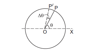Figure 4o

Suppose a object \(P\) is moving in a circle of radius \(r\) (Figure 4o). Let \(O\) be the centre of the circle. Let \(O\) be the origin and \(O X\) the \(X\)-axis. We call \(\theta\) the angular position of the object \(P\). As the object moves on the circle, from position \(P\) to \(P^{\prime}\) in time \(\Delta t\) the line \( O P\) turns through an angle \(\Delta \theta\) as shown in the figure 4o. \(\Delta \theta\) is called the angular distance. 

The rate of change of angular position (displacement) is called angular velocity. Thus, the angular velocity is

\(\omega=\lim _{\Delta t \rightarrow 0} \frac{\Delta \theta}{\Delta t}=\frac{d \theta}{d t}\)

Now, if the distance travelled by the object during the time \(\Delta t\) is \(\Delta \mathrm{s}\), i.e. \(P P^{\prime}\) is \(\Delta \mathrm{s}\), then speed of the object:
\(
v=\frac{\Delta s}{\Delta t}
\)
but \(\Delta s=r \Delta \theta\). Therefore :
\(
\begin{gathered}
v=r \frac{\Delta \theta}{\Delta t}=\mathrm{r} \omega \\
v=r \omega
\end{gathered}
\)
We can express centripetal acceleration \(a_{c}\) in terms of angular speed as

\(\begin{aligned}
&a_{c}=\frac{v^{2}}{r}=\frac{\omega^{2} R^{2}}{r}=\omega^{2} r \\
&a_{c}=\omega^{2} r
\end{aligned}\)

The time taken by an object to make one revolution is known as its time period \(T\) and the number of revolution made in one second is called its frequency \(f(=1 / T)\). However, during this time the distance moved by the object is \(s=2 \pi r\).
Therefore, \(v=2 \pi r / T=2 \pi r f\)
In terms of frequency \(v\), we have
\(
\begin{gathered}
\omega=2 \pi f \\
v=2 \pi r f \\
a_{c}=4 \pi^{2} f^{2} r
\end{gathered}
\)

Angular acceleration

The rate of change of angular velocity is called angular acceleration. Thus, the angular acceleration is
\(
\alpha=\frac{d \omega}{d t}=\frac{d^{2} \theta}{d t^{2}}
\)
If the angular acceleration \(\alpha\) is constant, we have
\(
\begin{aligned}
&\theta=\omega_{0} t+\frac{1}{2} \alpha t^{2} \\
&\omega=\omega_{0}+\alpha t
\end{aligned}
\)
and
\(\omega^{2}=\omega_{0}^{2}+2 \alpha \theta\)
where \(\omega_{0}\) and \(\omega\) are the angular velocities at \(t=0\) and at time \(t\) and \(\theta\) is the angular position at time \(t\).

Tangential acceleration

The direction of velocity \(v\) is along the tangent to the circle at every point. We know that the \(v\) is the linear speed of the object and is given by

\(v=r \omega\)

Differentiating equation the above equation with respect to time, the rate of change of speed is
\(
\begin{aligned}
\text { or, } \quad & a_{t}=\frac{d v}{d t}=r \frac{d \omega}{d t} \\
a_{t} &=r \alpha .
\end{aligned}
\)
Remember that \(a_{t}=\frac{d v}{d t}\) is the rate of change of speed and is not the rate of the change of velocity. It is, therefore, not equal to the net acceleration.

We should remember that \(a_{t}\) is called the tangential acceleration along the tangent and hence we have used the suffix \(t\). 

Example: 4.8

A particle moves in a circle of radius \(20 \mathrm{~cm}\) with a linear speed of \(10 \mathrm{~m} / \mathrm{s}\). Find the angular velocity.
Solution: The angular velocity is
\(
\omega=\frac{v}{r}=\frac{10 \mathrm{~m} / \mathrm{s}}{20 \mathrm{~cm}}=50 \mathrm{rad} / \mathrm{s}
\)

Example: 4.9

A particle travels in a circle of radius \(20 \mathrm{~cm}\) at a speed that uniformly increases. If the speed changes from \(5.0 \mathrm{~m} / \mathrm{s}\) to \(6.0 \mathrm{~m} / \mathrm{s}\) in \(2.0 \mathrm{~s}\), find the angular acceleration.
Solution: The tangential acceleration is given by
\(
\begin{aligned}
a_{t} &=\frac{d v}{d t}=\frac{v_{2}-v_{1}}{t_{2}-t_{1}} \\
&=\frac{6 \cdot 0-5 \cdot 0}{2 \cdot 0} \mathrm{~m} / \mathrm{s}^{2}=0.5 \mathrm{~m} / \mathrm{s}^{2} .
\end{aligned}
\)
The angular acceleration is \(\alpha=a_{t} / r\)
\(
=\frac{0.5 \mathrm{~m} / \mathrm{s}^{2}}{20 \mathrm{~cm}}=2.5 \mathrm{rad} / \mathrm{s}^{2} \text {. }
\)

UNIT VECTORS ALONG THE RADIUS AND THE TANGENT

Let’s calculate the \(e_{r}\) known as the radial unit vector and \(\overrightarrow{e_{t}}\) the tangential unit vector along the radius of a circle. Consider an object moving in a circle with the origin at \(O\) and, the line \(O X\) as the \(X\)-axis and a perpendicular radius \(O Y\) as the \(Y\)-axis. The angular position of the object at the point \(P\) is \(\theta\).

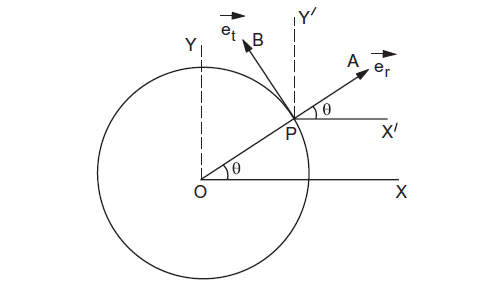Figure 4p

 

Draw a unit vector \(\overrightarrow{P A}=\overrightarrow{e_{r}}\) along the outward radius and a unit vector \(\overrightarrow{P B}=\overrightarrow{e_{t}}\) along the tangent in the direction of increasing \(\theta\). We call \(\overrightarrow{e_{r}}\) the radial unit vector and \(\overrightarrow{e_{t}}\) the tangential unit vector. Draw \(P X^{\prime}\) parallel to the \(X\)-axis and \(P Y^{\prime}\) parallel to the \(Y\)-axis. From the figure 4p,

\(\overrightarrow{P A}=\vec{i} P A \cos \theta+\vec{j} P A \sin \theta\)
or, \(\quad \overrightarrow{e_{r}}=\vec{i} \cos \theta+\vec{j} \sin \theta\). …………….. (4.1)

where \(\vec{i}\) and \(\vec{j}\) are the unit vectors along the \(X\) and \(Y\) axes respectively. Similarly,
\(\overrightarrow{P B}=-\vec{i} P B \sin \theta+\vec{j} P B \cos \theta\)
or, \(\quad \overrightarrow{e_{t}}=-\vec{i} \sin \theta+\vec{j} \cos \theta\). …………….. (4.2)

ACCELERATION IN CIRCULAR MOTION

From Figure 4p, It is clear that the position vector of the object at time \(t\) is
\(
\begin{aligned}
\vec{r} &=\overrightarrow{O P}=O P \overrightarrow{e_{r}} \\
&=r(\vec{i} \cos \theta+\vec{j} \sin \theta) \ldots \ldots \text { (4.3) }
\end{aligned} \)
Differentiating equation (4.3) with respect to time, the velocity of the object at time \(t\) is
\(
\begin{aligned}
\vec{v}=\frac{d \vec{r}}{d t} &=\frac{d}{d t}[r(\vec{i} \cos \theta+\vec{j} \sin \theta)] \\
&=r\left[\vec{i}\left(-\sin \theta \frac{d \theta}{d t}\right)+\vec{j}\left(\cos \theta \frac{d \theta}{d t}\right)\right] \\
&=r \omega[-\vec{i} \sin \theta+\vec{j} \cos \theta] \ldots \ldots \text { (4.4) }
\end{aligned} \)

The term \(r \omega\) is the speed of the object at time \(t\) (\(v=r \omega\)) and the vector in the square bracket is the unit vector \(\overrightarrow{e_{t}}\) along the tangent. Thus, the velocity of the object at any instant is along the tangent to the circle and its magnitude is \(v=r \omega\).

The acceleration of the object at time \(t\) is \(\vec{a}=\frac{d \vec{v}}{d t} \cdot\) From (equation 4.4),
\(
\begin{aligned}
\vec{a} &=r\left[\omega \frac{d}{d t}[-\vec{i} \sin \theta+\vec{j} \cos \theta]+\frac{d \omega}{d t}[-\vec{i} \sin \theta+\vec{j} \cos \theta]\right] \\
&=\omega r\left[-\vec{i} \cos \theta \frac{d \theta}{d t}-\vec{j} \sin \theta \frac{d \theta}{d t}\right]+r \frac{d \omega}{d t} \overrightarrow{e_{t}} \\
&=-\omega^{2} r[\vec{i} \cos \theta+\vec{j} \sin \theta]+r \frac{d \omega}{d t} \overrightarrow{e_{t}} \\
&=-\omega^{2} r \overrightarrow{e_{r}}+\frac{d v}{d t} \overrightarrow{e_{t}} \ldots \ldots \text { (4.5) }
\end{aligned}\)
where \(\overrightarrow{e_{r}}\) and \(\overrightarrow{e_{t}}\) are the unit vectors along the radial and tangential directions respectively and \(v\) is the speed of the objectat time \(t\). We have used
\(
r \frac{d \omega}{d t}=\frac{d}{d t}(r \omega)=\frac{d v}{d t} .
\)

Example: 4.10

Prove that if an object moves in a circle of radius \(r\) with a constant speed \(v\), its acceleration is \(v^{2} / r\) directed towards the centre. 

Solution: If a particle moves in the circle with a uniform speed, we call it a uniform circular motion. In this case, \(\frac{d v}{d t}=0\) and equation (4.5) gives
\(\vec{a}=-\omega^{2} r \overrightarrow{e_{r}}\)
Thus, the acceleration of the particle is in the direction of \(-\overrightarrow{e_{r}}\), that is, towards the centre. The magnitude of the acceleration is
\(
\begin{aligned}
a_{r} &=\omega^{2} r \\
&=\frac{v^{2}}{r^{2}} r=\frac{v^{2}}{r}
\end{aligned}\)

[ Note: some books use the notation \(a_{c}\) instead of \(a_{r}\) ]

Thus, if a particle moves in a circle of radius \(r\) with a constant speed \(v\), its acceleration is \(v^{2} / r\) directed towards the centre known as the centripetal acceleration. Note that the speed remains constant, the direction continuously changes, and hence the “velocity” changes and there is an acceleration during the motion.

Example: 4.11

Find the magnitude of the linear acceleration of a particle moving in a circle of radius \(10 \mathrm{~cm}\) with uniform speed completing the circle in \(4 \mathrm{~s}\).

Solution: The distance covered in completing the circle is \(2 \pi r=2 \pi \times 10 \mathrm{~cm}\). The linear speed is \(v=2 \pi r / t=\frac{2 \pi \times 10 \mathrm{~cm}}{4 \mathrm{~s}}=5 \pi \mathrm{cm} / \mathrm{s}.\)
The linear acceleration is
\(
a=\frac{v^{2}}{r}=\frac{(5 \pi \mathrm{cm} / \mathrm{s})^{2}}{10 \mathrm{~cm}}=2.5 \pi^{2} \mathrm{~cm} / \mathrm{s}^{2} \text {. }
\)
This acceleration is directed towards the centre of the circle.

Nonuniform Circular Motion

If the speed of the object moving in a circle is not constant, the acceleration has both the radial and the tangential components. According to equation (4.5), the radial and the tangential accelerations are
and \(\quad a_{r}=-\omega^{2} r=-v^{2} / r \text { and } \quad a_{t}=\frac{d v}{d t} \ldots \ldots \text { (4.6) }\) 
Thus, the component of the acceleration towards the centre is \(\omega^{2} r=v^{2} / r\) and the component along the tangent (along the direction of motion) is \(d v / d t\). The magnitude of the acceleration is
\(
a=\sqrt{a_{r}^{2}+a_{t}^{2}}=\sqrt{\left(\frac{v^{2}}{r}\right)^{2}+\left(\frac{d v}{d t}\right)^{2}}
\)

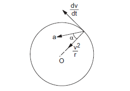Figure 4q

The direction of this resultant acceleration makes an angle \(\alpha\) with the radius (figure 4q) where
\(
\tan \alpha=\left(\frac{d v}{d t}\right) /\left(\frac{v^{2}}{r}\right) .
\)

Example: 4.12

An object moves in a circle of radius \(20 \mathrm{~cm}\). It’s linear speed is given by \(v=2 t\), where \(t\) is in second and \(v\) in metre/second. Find the radial and tangential acceleration at \(t=3 \mathrm{~s}\).

Solution: The linear speed at \(t=3 \mathrm{~s}\) is
\(
v=2 t=6 \mathrm{~m} / \mathrm{s} \text {. }
\)
The radial acceleration at \(t=3 \mathrm{~s}\) is
\(
a_{r}=v^{2} / r=\frac{36 \mathrm{~m}^{2} / \mathrm{s}^{2}}{0 \cdot 20 \mathrm{~m}}=180 \mathrm{~m} / \mathrm{s}^{2} \text {. }
\)

The tangential acceleration is \(a_{t}=\frac{d v}{d t}=\frac{d(2 t)}{d t}=2 \mathrm{~m} / \mathrm{s}^{2} .\)

Centripetal Force

If an object moves in a circle as seen from an inertial frame, a resultant nonzero force must act on the particle. That is because an object moving in a circle is accelerated and acceleration can be produced in an inertial frame only if a resultant force acts on it. If the speed of the object remains constant, the acceleration of the object is towards the centre and its magnitude is \(v^{2} / r\). Here \(v\) is the speed of the object and \(r\) is the radius of the circle. The resultant force must act towards the centre and its magnitude \(F\) must satisfy
\(a=\frac{F}{m}\)
\(\frac{v^{2}}{r}=\frac{F}{m}\)
\(F=\frac{m v^{2}}{r} \ldots \ldots \text { (4.7) }\).
Since this resultant force is directed towards the centre, it is called centripetal force. Thus, a centripetal force of magnitude \(m v^{2} / r\) is needed to keep the object in a uniform circular motion.

CIRCULAR TURNINGS AND BANKING OF ROADS

When there is no friction the vertical component of the road acts as a normal force due to which the weight of the vehicle is balanced and the horizontal component gives in to the centripetal force in the direction of the centre of the curvature of the road. The inclination occurs at the horizontal and longitudinal axis. 

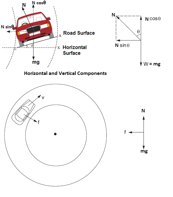Figure 4r

Consider a car of mass \(m\) moving at a speed \(v\) is making a turn on the circular path of radius \(r\). Let \(\theta\) be the banking angle and \(f\) be the frictional force acting between the road and the car’s tires. The external forces acting on the vehicle are
(i) weight \(mg\)
(ii) Normal contact force \(N\) and
(iii) friction \(f\)

If the road is horizontal, the normal force \(N\) is vertically upward. The only horizontal force that can act towards the centre is the friction \(f\). The tires get a tendency to skid outward and the frictional force which opposes this skidding acts towards the centre. Thus, for a safe turn, we must have
\(\frac{v^{2}}{r}=\frac{f}{m}\)
or, \(\quad f=\frac{m v^{2}}{r}\)

However, there is a limit to the magnitude of the frictional force. If \(\mu_{s}\) is the coefficient of static friction between the tires and the road, the magnitude of friction \(f\) cannot exceed \(\mu_{s} N\). For vertical equilibrium \(N=mg\), so that
\(f \leq \mu_{s} mg\)
Thus, for a safe turn
\(\frac{m v^{2}}{r} \leq \mu_{s} mg\)

Therefore, \(\quad \mu_{s} \geq \frac{v^{2}}{r g}\).

Friction is not always reliable at circular turns if high speeds and sharp turns are involved. To avoid dependence on friction, the roads are banked at the turn so that the outer part of the road is somewhat lifted up as compared to the inner part (figure 4r). 

The surface of the road makes an angle \(\theta\) with the horizontal throughout the turn. The normal force \(N\) makes an angle \(\theta\) with the vertical. At the correct speed, the horizontal component of \(N\) is sufficient to produce the acceleration towards the centre and the self-adjustable frictional force keeps its value zero.

\(N \cos \theta \rightarrow\) Normal reaction along the vertical axis

\(\mathrm{f} \sin \theta \rightarrow\) Frictional force along the vertical axis

\(\mathrm{mg} \rightarrow\) Weight of the vehicle acting downwards

Applying Newton’s second law along the radius and the first law in the vertical direction,
\(\Rightarrow N \sin \theta=\frac{m v^{2}}{r}\)
and, \(N \cos \theta=mg \)
These equations give, \(\tan \theta=\frac{v^{2}}{r g}\); \(\theta=\tan ^{-1} \frac{v^{2}}{r g} \ldots \ldots \text { (4.8) }\)

The angle \(\theta\) depends on the speed of the vehicle as well as on the radius of the turn. If the speed of the car is a little less or a little more than the correct speed, the self-adjustable static friction operates between the tires and the road, and the vehicle does not skid or slip. If the speed is too different from that given by equation (4.8), even the maximum friction cannot prevent a skid or a slip.

Example: 4.13

The road at a circular turn of radius \(10 \mathrm{~m}\) is banked by an angle of \(10^{\circ}\). With what speed should a vehicle move on the turn so that the normal contact force is able to provide the necessary centripetal force?
Solution:  If \(v\) is the correct speed,
\(\tan \theta=\frac{v^{2}}{r g}\)

\(\quad \begin{aligned}
v &=\sqrt{r g \tan \theta} \\
&=\sqrt{(10 \mathrm{~m})\left(9.8 \mathrm{~m} / \mathrm{s}^{2}\right)\left(\tan 10^{\circ}\right)}=4 \cdot 2 \mathrm{~m} / \mathrm{s}
\end{aligned}\)

CENTRIFUGAL FORCE

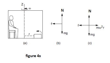
Let us assume an observer is sitting in a closed cabin which is made to rotate about the vertical \(Z\)-axis at a uniform angular velocity \(\omega\) (figure 4s). The \(X\) and \(Y\) axes are fixed in the cabin. Consider a heavy box of mass \(m\) kept on the floor at a distance \(r\) from the \(Z\)-axis. Suppose the floor and the box are rough and the box does not slip on the floor as the cabin rotates. The box is at rest with respect to the cabin and hence is rotating with respect to the ground at an angular velocity \(\omega\). Let us first analyze the motion of the box from the ground frame. In this frame (which is inertial) the box is moving in a circle of radius \(r\). It, therefore, has an acceleration \(v^{2} / r=\omega^{2} r\) towards the centre. The resultant force on the box must be towards the centre and its magnitude must be \(m \omega^{2} r\). The forces on the box are
(i) weight \(mg\)
(ii) normal force\(N\) by the floor
(iii) friction \(f\) by the floor.
Figure (4s) shows the free body diagram for the box. Since the resultant is towards the centre and its magnitude is \(m \omega^{2} r\), we should have
\(f=m \omega^{2} r\)

The floor exerts a force of static friction \(f=m \omega^{2} r\) towards the origin.

When we observe the same box from the frame of the rotating cabin. The observer there finds that the box is at rest. If we apply Newton’s laws, the resultant force on the box should be zero. The weight and the normal contact force balance each other but the frictional force \(f=m \omega^{2} r\) acts on the box towards the origin. To make the resultant zero, a pseudo force must be assumed which acts on the box away from the centre (radially outward) and has a magnitude \(m \omega^{2} r\). This pseudo force is called the centrifugal force. Therefore, the Centrifugal force = \(m \omega^{2} r\).
The free-body diagram is shown in figure 4s-c. As the box is at rest, Newton’s first law gives
\(f=m \omega^{2} r\)

EFFECT OF EARTH’S ROTATION ON APPARENT WEIGHT

The earth rotates about its axis at an angular speed of one revolution in 24 hours. The line joining the north and the south poles is the axis of rotation. Every point on the earth moves in a circle. A point at the equator moves in a circle of radius equal to the radius of the earth and the centre of the circle is same as the centre of the earth. Consider a place \(P\) on the earth (figure 4t).

 

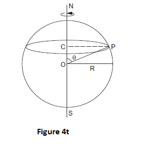
Drop a perpendicular \(P C\) from \(P\) to the axis \(S N\). The place \(P\) rotates in a circle with the centre at \(C\). The radius of this circle is \(C P(r)\). The angle between the axis \(S N\) and the radius \(O P\) through \(P\) is called the colatitude of the place \(P\). We have
\(
\begin{aligned}
C P &=O P \sin \theta \\
r &=R \sin \theta
\end{aligned}
\)
\(
\text { or, } \quad r=R \sin \theta
\); where \(R\) is the radius of the earth.
If we work from the frame of reference of the earth, we shall have to assume the existence of the pseudo forces. In particular, a centrifugal force \(m \omega^{2} r\) has to be assumed on any particle of mass \(m\) placed at \(P\). Here \(\omega\) is the angular speed of the earth. If we discuss the equilibrium of bodies at rest in the earth’s frame, no other pseudo force is needed.

Consider a heavy particle of mass \(m\) suspended through a string from the ceiling of a laboratory at colatitude \(\theta\) (figure 4u). Looking from the earth’s frame the particle is in equilibrium and the forces on it are
(a) gravitational attraction \(mg\) towards the centre of the earth, i.e., vertically downward.

(b) centrifugal force \(m \omega^{2} r\) towards \(C P\) and

(c) the tension in the string \(T\) along the string.

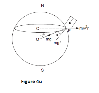
As the particle is in equilibrium (in the frame of earth), the three forces on the particle should add up to zero.
The resultant of \(mg\) and \(m \omega^{2} r\)
\(
\begin{aligned}
&=\sqrt{(m g)^{2}+\left(m \omega^{2} r\right)^{2}+2(m g)\left(m \omega^{2} r\right) \cos \left(90^{\circ}+\theta\right)} \\
&=m \sqrt{g^{2}+\omega^{4} R{ }^{2} \sin ^{2} \theta-2 g \omega^{2} R \sin ^{2} \theta} \\
&=m g^{\prime}
\end{aligned}
\)

where \(g^{\prime}=\sqrt{g^{2}-\omega^{2} R \sin ^{2} \theta\left(2 g-\omega^{2} R\right)}\ldots(4.9)\)
Also, the direction of this resultant makes an angle \(\alpha\) with the vertical \(O P\), where
\(
\begin{aligned}
\tan \alpha &=\frac{m \omega^{2} r \sin \left(90^{\circ}+\theta\right)}{m g+m \omega^{2} r \cos \left(90^{\circ}+\theta\right)} \\
&=\frac{\omega^{2} R \sin \theta \cos \theta}{g-\omega^{2} R \sin ^{2} \theta}\end{aligned} \ldots(4.10)\)

As the three forces acting on the particle must add up to zero, the force of tension must be equal and opposite to the resultant of the rest two. Thus, the magnitude of the tension in the string must be \(m g^{\prime}\) and the direction of the string should make an angle \(\alpha\) with the true vertical.

The magnitude of \(g^{\prime}\) is also different from \(g\). As \(2 g>\omega^{2} R\), it is clear from equation (4.9) that \(g^{\prime}<g\). One way of measuring the weight of a body is to suspend it by a string and find the tension in the string. The tension itself is taken as a measure of the weight. As \(T=m g^{\prime}\), the weight so observed is less than the true weight mg. This is known as the apparent weight. Similarly, if a person stands on the platform of a weighing machine, the platform exerts a normal force \(N\) which is equal to \(m g^{\prime}\). The reading of the machine responds to the force exerted on it and hence the weight recorded is the apparent weight \(m g^{\prime}\).
At equator, \(\theta=90^{\circ}\) and equation (4.9) gives
\(
\begin{aligned}
g^{\prime} &=\sqrt{g^{2}-2 g \omega{ }^{2} R+\omega{ }^{4} R{ }^{2}} \\
&=g-\omega{ }^{2} R \\
\text { or, } \quad m g^{\prime} &=m g-m \omega{ }^{2} R .
\end{aligned}
\)
This can be obtained in a more straightforward way. At the equator, \(m \omega{ }^{2} R\) is directly opposite to \(mg\) and the resultant is simply \(mg-m \omega^{2} R\). Also, this resultant is towards the centre of the earth so that at the equator the plumb line stands along the true vertical.

At poles, \(\theta=0\) and equation (4.9) gives \(g^{\prime}=g\) and equation (4.10) shows that \(\alpha=0\). Thus, there is no apparent change in \(g\) at the poles. This is because the poles themselves do not rotate and hence the effect of the earth’s rotation is not felt there.

Example: 4.14

A body weighs \(98 \mathrm{~N}\) on a spring balance at the north pole. What will be its weight recorded on the same scale if it is shifted to the equator? Use \(g=G M / R^{2}=9.8 \mathrm{~m} / \mathrm{s}^{2}\) and the radius of the earth \(R=6400 \mathrm{~km}\).

Solution: At the poles, the apparent weight is the same as the true weight. Thus,
\(
\begin{aligned}
& 98 \mathrm{~N} &=m g=m\left(9 \cdot 8 \mathrm{~m} / \mathrm{s}^{2}\right) \\
\text { or, } & m &=10 \mathrm{~kg} .
\end{aligned}
\)
At the equator, the apparent weight is
\(m g^{\prime}=m g-m \omega{ }^{2} R \text {. }\)
The radius of the earth is \(6400 \mathrm{~km}\) and the angular speed is
\(
\omega=\frac{2 \pi \mathrm{rad}}{24 \times 60 \times 60 \mathrm{~s}}=7 \cdot 27 \times 10^{-5} \mathrm{rad} / \mathrm{s}
\)
Thus,
\(
\begin{aligned}
m g^{\prime} &=98 \mathrm{~N}-(10 \mathrm{~kg})\left(7 \cdot 27 \times 10^{-5} \mathrm{~s}^{-1}\right)^{2}(6400 \mathrm{~km}) \\
&=97 \cdot 66 \mathrm{~N} .
\end{aligned}
\)